Advanced Workflows

Standard regression analysis assumes independent observations and constant effects across subgroups. In practice, these assumptions often fail: observations may be clustered (e.g., subjects within study sites), effects may vary by subgroup (interaction), or the baseline hazard may differ across strata. This vignette demonstrates advanced analytical techniques to address these complexities.

Preliminaries

The examples in this vignette use the clintrial dataset included with summata:

library(summata)
library(survival)
library(ggplot2)

data(clintrial)
data(clintrial_labels)

# Examine the clustering structure
table(clintrial$site)
##> 
##>   Site Alpha    Site Beta   Site Gamma   Site Delta Site Epsilon    Site Zeta     Site Eta   Site Theta    Site Iota   Site Kappa 
##>           76           80           72           89           86           93           89           75          102           88

The clintrial dataset includes 10 study sites, providing a natural clustering variable for hierarchical analysis.

n.b.: To ensure correct font rendering and figure sizing, the forest plots below are displayed using a helper function (queue_plot()) that applies each plot’s recommended dimensions (stored in the "rec_dims" attribute) via the ragg graphics device. In practice, replace queue_plot() with ggplot2::ggsave() using recommended plot dimensions for equivalent results:
p <- glmforest(model, data = mydata)
dims <- attr(p, "rec_dims")
ggplot2::ggsave("forest_plot.png", p,
                width = dims$width, 
                height = dims$height)
This ensures that the figure size is always large enough to accommodate the constituent plot text and graphics, and it is generally the preferred method for saving forest plot outputs in summata.

Interaction Effects

Interaction analysis tests whether the association between a predictor and outcome varies across levels of another variable. Interactions are specified using colon notation in the interactions parameter; main effects are automatically included alongside the interaction term.

Example 1: Two-Way Interaction

Specify interactions using colon notation in the interactions parameter:

example1 <- fit(
  data = clintrial,
  outcome = "surgery",
  predictors = c("age", "sex", "treatment", "stage"),
  interactions = c("sex:treatment"),
  model_type = "glm",
  labels = clintrial_labels
)

example1
##> 
##> Multivariable Logistic Model
##> Formula: surgery ~ age + sex + treatment + stage + sex:treatment
##> n = 847, Events = 368
##> 
##>                                  Variable   Group      n Events     aOR (95% CI) p-value
##>                                    <char>  <char> <char> <char>           <char>  <char>
##>  1:                           Age (years)       -    847    368 0.96 (0.94-0.97) < 0.001
##>  2:                                   Sex  Female    449    203        reference       -
##>  3:                                          Male    398    165 1.01 (0.55-1.87)   0.968
##>  4:                       Treatment Group Control    194     93        reference       -
##>  5:                                        Drug A    292    173 2.09 (1.20-3.62)   0.009
##>  6:                                        Drug B    361    102 0.50 (0.29-0.87)   0.013
##>  7:                         Disease Stage       I    211    125        reference       -
##>  8:                                            II    263    133 0.69 (0.47-1.03)   0.069
##>  9:                                           III    241     91 0.41 (0.27-0.62) < 0.001
##> 10:                                            IV    132     19 0.09 (0.05-0.16) < 0.001
##> 11: Sex (Male) × Treatment Group (Drug A)       -    128     73 0.77 (0.34-1.71)   0.515
##> 12: Sex (Male) × Treatment Group (Drug B)       -    175     49 0.79 (0.36-1.73)   0.554

Example 2: Multiple Interactions

Test multiple effect modifiers simultaneously:

example2 <- fit(
  data = clintrial,
  outcome = "Surv(os_months, os_status)",
  predictors = c("age", "sex", "treatment", "stage"),
  interactions = c("sex:treatment", "stage:treatment"),
  model_type = "coxph",
  labels = clintrial_labels
)

example2
##> 
##> Multivariable Cox PH Model
##> Formula: Surv(os_months, os_status) ~ age + sex + treatment + stage + sex:treatment + stage:treatment
##> n = 847, Events = 606
##> 
##>                                           Variable   Group      n Events     aHR (95% CI) p-value
##>                                             <char>  <char> <char> <char>           <char>  <char>
##>  1:                                    Age (years)       -    847    606 1.04 (1.03-1.04) < 0.001
##>  2:                                            Sex  Female    450    298        reference       -
##>  3:                                                   Male    400    311 1.32 (0.95-1.83)   0.094
##>  4:                                Treatment Group Control    196    151        reference       -
##>  5:                                                 Drug A    292    184 0.70 (0.43-1.14)   0.153
##>  6:                                                 Drug B    362    274 0.67 (0.41-1.09)   0.106
##>  7:                                  Disease Stage       I    211    127        reference       -
##>  8:                                                     II    263    172 1.11 (0.73-1.70)   0.624
##>  9:                                                    III    241    186 1.94 (1.21-3.09)   0.006
##> 10:                                                     IV    132    121 3.69 (2.28-5.97) < 0.001
##> 11:          Sex (Male) × Treatment Group (Drug A)       -    128     89 1.11 (0.72-1.72)   0.637
##> 12:          Sex (Male) × Treatment Group (Drug B)       -    176    143 0.98 (0.65-1.46)   0.903
##> 13:  Treatment Group (Drug A) × Disease Stage (II)       -     93     52 0.75 (0.42-1.35)   0.339
##> 14: Treatment Group (Drug A) × Disease Stage (III)       -     75     50 0.65 (0.35-1.20)   0.171
##> 15:  Treatment Group (Drug A) × Disease Stage (IV)       -     46     37 0.70 (0.37-1.34)   0.287
##> 16:  Treatment Group (Drug B) × Disease Stage (II)       -    105     73 1.37 (0.78-2.42)   0.278
##> 17: Treatment Group (Drug B) × Disease Stage (III)       -    127    103 1.30 (0.72-2.35)   0.375
##> 18:  Treatment Group (Drug B) × Disease Stage (IV)       -     55     54 1.24 (0.66-2.31)   0.504

Example 3: Continuous × Categorical Interaction

Test whether effects of a continuous variable vary by group:

example3 <- fit(
  data = clintrial,
  outcome = "los_days",
  predictors = c("age", "sex", "treatment", "stage", "surgery"),
  interactions = c("age:treatment"),
  model_type = "lm",
  labels = clintrial_labels
)

example3
##> 
##> Multivariable Linear Model
##> Formula: los_days ~ age + sex + treatment + stage + surgery + age:treatment
##> n = 827
##> 
##>                                   Variable   Group      n Adj. Coefficient (95% CI) p-value
##>                                     <char>  <char> <char>                    <char>  <char>
##>  1:                            Age (years)       -    827       0.14 (0.09 to 0.19) < 0.001
##>  2:                                    Sex  Female    441                 reference       -
##>  3:                                           Male    386       0.99 (0.46 to 1.52) < 0.001
##>  4:                        Treatment Group Control    190                 reference       -
##>  5:                                         Drug A    288     -2.39 (-6.00 to 1.23)   0.197
##>  6:                                         Drug B    349      0.03 (-3.51 to 3.58)   0.985
##>  7:                          Disease Stage       I    207                 reference       -
##>  8:                                             II    259       1.33 (0.62 to 2.04) < 0.001
##>  9:                                            III    235       3.10 (2.36 to 3.84) < 0.001
##> 10:                                             IV    126       4.32 (3.42 to 5.22) < 0.001
##> 11:                     Surgical Resection      No    459                 reference       -
##> 12:                                            Yes    368       3.29 (2.69 to 3.88) < 0.001
##> 13: Age (years) × Treatment Group (Drug A)       -    288      0.02 (-0.04 to 0.08)   0.557
##> 14: Age (years) × Treatment Group (Drug B)       -    349      0.05 (-0.01 to 0.11)   0.114

Example 4: Interaction in fullfit()

Include interaction terms in combined univariable/multivariable analysis:

example4 <- fullfit(
  data = clintrial,
  outcome = "surgery",
  predictors = c("age", "sex", "treatment", "stage", "sex:treatment"),
  model_type = "glm",
  method = "all",
  labels = clintrial_labels
)

example4
##> 
##> Fullfit Analysis Results
##> Outcome: surgery
##> Model Type: glm
##> Method: all
##> Predictors Screened: 5
##> Multivariable Predictors: 5
##> 
##>                                     Variable   Group      n Events      OR (95% CI)   Uni p     aOR (95% CI) Multi p
##>                                       <char>  <char> <char> <char>           <char>  <char>           <char>  <char>
##>  1:                              Age (years)       -    850    370 0.96 (0.95-0.98) < 0.001 0.96 (0.94-0.97) < 0.001
##>  2:                                      Sex  Female    450    204        reference       -        reference       -
##>  3:                                             Male    400    166 0.86 (0.65-1.12)   0.261 1.01 (0.55-1.87)   0.968
##>  4:                          Treatment Group Control    196     94        reference       -        reference       -
##>  5:                                           Drug A    292    173 1.58 (1.10-2.27)   0.014 2.09 (1.20-3.62)   0.009
##>  6:                                           Drug B    362    103 0.43 (0.30-0.62) < 0.001 0.50 (0.29-0.87)   0.013
##>  7:                            Disease Stage       I    211    125        reference       -        reference       -
##>  8:                                               II    263    133 0.70 (0.49-1.01)   0.060 0.69 (0.47-1.03)   0.069
##>  9:                                              III    241     91 0.42 (0.29-0.61) < 0.001 0.41 (0.27-0.62) < 0.001
##> 10:                                               IV    132     19 0.12 (0.07-0.20) < 0.001 0.09 (0.05-0.16) < 0.001
##> 11: Sex (Female) × Treatment Group (Control)       -    100     51 2.62 (1.57-4.37) < 0.001                -       -
##> 12:   Sex (Male) × Treatment Group (Control)       -     96     43 2.04 (1.22-3.43)   0.007                -       -
##> 13:  Sex (Female) × Treatment Group (Drug A)       -    164    100 3.94 (2.50-6.20) < 0.001                -       -
##> 14:    Sex (Male) × Treatment Group (Drug A)       -    128     73 3.34 (2.07-5.40) < 0.001 0.77 (0.34-1.71)   0.515
##> 15:  Sex (Female) × Treatment Group (Drug B)       -    186     53 1.00 (0.64-1.59)   0.986                -       -

Example 5: Testing Interaction Significance

Use compfit() to formally evaluate whether interactions improve model fit (see Model Comparison):

example5 <- compfit(
  data = clintrial,
  outcome = "surgery",
  model_list = list(
    "Main Effects" = c("age", "sex", "treatment", "stage"),
    "Sex × Treatment" = c("age", "sex", "treatment", "stage"),
    "Stage × Treatment" = c("age", "sex", "treatment", "stage"),
    "Both Interactions" = c("age", "sex", "treatment", "stage")
  ),
  interactions_list = list(
    NULL,
    c("sex:treatment"),
    c("stage:treatment"),
    c("sex:treatment", "stage:treatment")
  ),
  model_type = "glm",
  labels = clintrial_labels
)

example5
##> 
##> Model Comparison Results
##> Outcome: surgery
##> Model Type: glm
##> 
##> CMS Weights:
##>   Convergence: 15%
##>   AIC: 25%
##>   Concordance: 40%
##>   Pseudo-R²: 15%
##>   Brier score: 5%
##> 
##> Recommended Model: Main Effects (CMS: 75.4)
##> 
##> Models ranked by selection score:
##>                Model   CMS     N Events Predictors Converged   AIC    BIC Pseudo-R² Concordance Brier Score Global p
##>               <char> <num> <int>  <num>      <int>    <char> <num>  <num>     <num>       <num>       <num>   <char>
##> 1:      Main Effects  75.4   847    368          4       Yes 984.4 1022.4     0.165       0.765       0.195  < 0.001
##> 2:   Sex × Treatment  68.6   847    368          4       Yes 987.9 1035.4     0.165       0.765       0.195  < 0.001
##> 3: Stage × Treatment  57.2   847    368          4       Yes 993.8 1060.1     0.167       0.766       0.194  < 0.001
##> 4: Both Interactions  50.6   847    368          4       Yes 997.2 1073.1     0.168       0.766       0.194  < 0.001
##> 
##> CMS interpretation: 85+ Excellent, 75-84 Very Good, 65-74 Good, 55-64 Fair, < 55 Poor

Example 6: Forest Plot with Interactions

Visualize models including interaction terms:

interaction_model <- fit(
  data = clintrial,
  outcome = "surgery",
  predictors = c("age", "sex", "treatment", "stage"),
  interactions = c("sex:treatment"),
  model_type = "glm",
  labels = clintrial_labels
)

example6 <- glmforest(
  x = attr(interaction_model, "model"),
  title = "Logistic Regression with Interaction",
  labels = clintrial_labels,
  indent_groups = TRUE,
  zebra_stripes = TRUE
)
queue_plot(example6)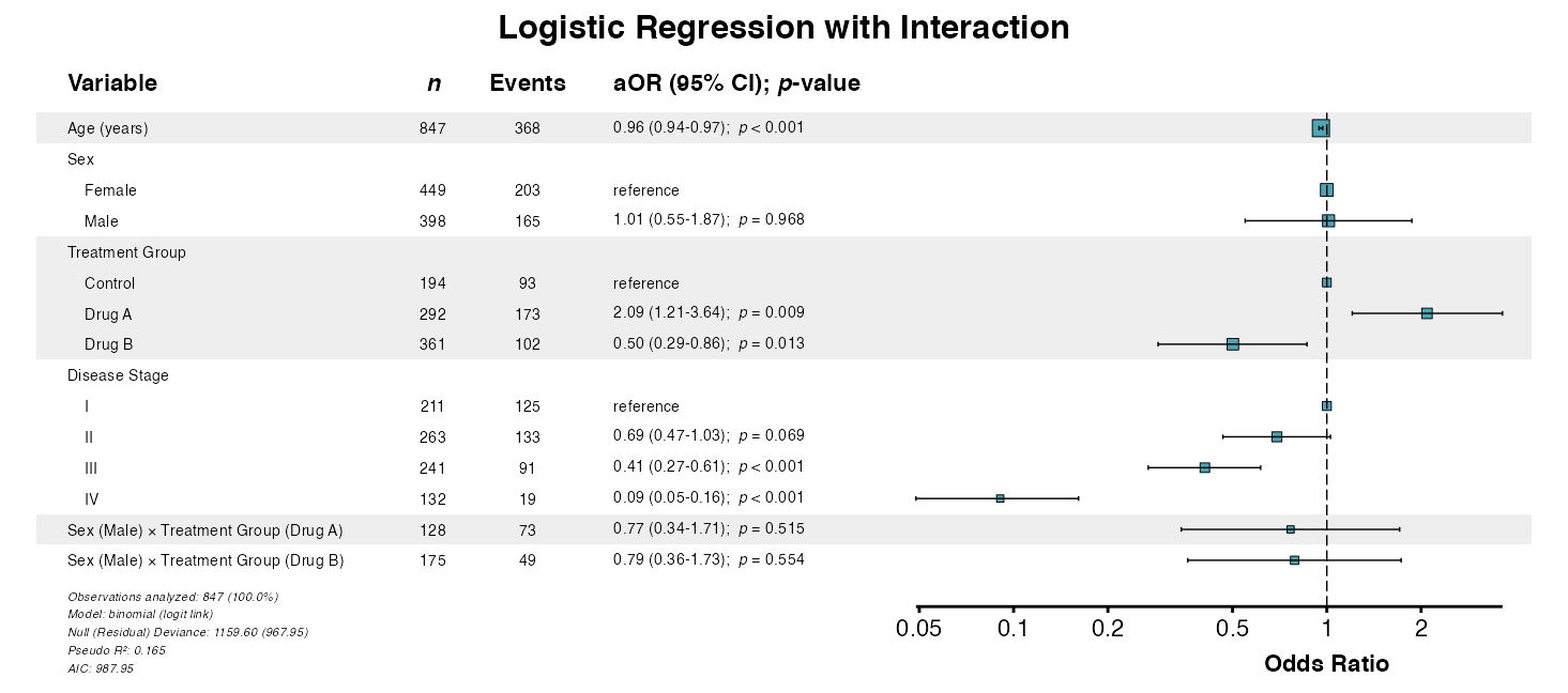

Mixed-Effects Models

Mixed-effects models (multilevel or hierarchical models) account for correlation within clusters by incorporating random effects. The summata package supports linear mixed models (lmer), generalized linear mixed models (glmer), and Cox mixed models (coxme).

Random effects are specified using pipe notation within either the predictors parameter or in a separate random parameter:

Syntax	Meaning
`(1\\|group)`	Random intercepts by group
`(x\\|group)`	Random intercepts and slopes for x
`(1\\|g1) + (1\\|g2)`	Crossed random effects

Example 7: Random Intercepts (Linear Mixed)

The (1|site) syntax specifies a random intercept for each site:

example7 <- fit(
  data = clintrial,
  outcome = "los_days",
  predictors = c("age", "sex", "treatment", "stage", "(1|site)"),
  model_type = "lmer",
  labels = clintrial_labels
)

example7
##> 
##> Multivariable Linear Mixed Model
##> Formula: los_days ~ age + sex + treatment + stage + (1|site)
##> n = 827
##> 
##>            Variable   Group      n Adj. Coefficient (95% CI) p-value
##>              <char>  <char> <char>                    <char>  <char>
##>  1:     Age (years)       -    827       0.14 (0.11 to 0.16) < 0.001
##>  2:             Sex  Female    441                 reference       -
##>  3:                    Male    386       0.82 (0.28 to 1.37)   0.003
##>  4: Treatment Group Control    190                 reference       -
##>  5:                  Drug A    288    -0.94 (-1.68 to -0.20)   0.013
##>  6:                  Drug B    349       2.41 (1.70 to 3.13) < 0.001
##>  7:   Disease Stage       I    207                 reference       -
##>  8:                      II    259       1.25 (0.51 to 1.98) < 0.001
##>  9:                     III    235       2.43 (1.67 to 3.19) < 0.001
##> 10:                      IV    126       2.96 (2.07 to 3.85) < 0.001

Example 8: Random Intercepts (Logistic Mixed)

For binary outcomes with clustering (note the use of an independent random parameter):

example8 <- fit(
    data = clintrial,
    outcome = "surgery",
    predictors = c("age", "sex", "treatment", "stage"),
    random = "(1|site)",
    model_type = "glmer",
    labels = clintrial_labels
)

example8
##> 
##> Multivariable glmerMod Model
##> Formula: surgery ~ age + sex + treatment + stage + (1|site)
##> n = 847, Events = 368
##> 
##>            Variable   Group      n Events     aOR (95% CI) p-value
##>              <char>  <char> <char> <char>           <char>  <char>
##>  1:     Age (years)       -    847    368 0.96 (0.94-0.97) < 0.001
##>  2:             Sex  Female    449    203        reference       -
##>  3:                    Male    398    165 0.84 (0.62-1.14)   0.263
##>  4: Treatment Group Control    194     93        reference       -
##>  5:                  Drug A    292    173 1.84 (1.23-2.75)   0.003
##>  6:                  Drug B    361    102 0.45 (0.30-0.66) < 0.001
##>  7:   Disease Stage       I    211    125        reference       -
##>  8:                      II    263    133 0.69 (0.47-1.03)   0.070
##>  9:                     III    241     91 0.41 (0.27-0.62) < 0.001
##> 10:                      IV    132     19 0.09 (0.05-0.17) < 0.001

Example 9: Random Slopes

Allow effects to vary by cluster:

example9 <- fit(
  data = clintrial,
  outcome = "los_days",
  predictors = c("age", "sex", "treatment", "stage", "(1 + treatment|site)"),
  model_type = "lmer",
  labels = clintrial_labels
)

example9
##> 
##> Multivariable Linear Mixed Model
##> Formula: los_days ~ age + sex + treatment + stage + (1 + treatment|site)
##> n = 827
##> 
##>            Variable   Group      n Adj. Coefficient (95% CI) p-value
##>              <char>  <char> <char>                    <char>  <char>
##>  1:     Age (years)       -    827       0.14 (0.11 to 0.16) < 0.001
##>  2:             Sex  Female    441                 reference       -
##>  3:                    Male    386       0.83 (0.28 to 1.38)   0.003
##>  4: Treatment Group Control    190                 reference       -
##>  5:                  Drug A    288    -0.95 (-1.81 to -0.09)   0.031
##>  6:                  Drug B    349       2.40 (1.65 to 3.16) < 0.001
##>  7:   Disease Stage       I    207                 reference       -
##>  8:                      II    259       1.27 (0.53 to 2.00) < 0.001
##>  9:                     III    235       2.44 (1.68 to 3.20) < 0.001
##> 10:                      IV    126       3.01 (2.12 to 3.90) < 0.001

Example 10: Cox Mixed-Effects Model

For survival outcomes with clustering:

example10 <- fit(
  data = clintrial,
  outcome = "Surv(os_months, os_status)",
  predictors = c("age", "sex", "treatment", "stage", "(1|site)"),
  model_type = "coxme",
  labels = clintrial_labels
)

example10
##> 
##> Multivariable Mixed Effects Cox Model
##> Formula: Surv(os_months, os_status) ~ age + sex + treatment + stage + (1|site)
##> n = 847, Events = 606
##> 
##>            Variable   Group      n Events     aHR (95% CI) p-value
##>              <char>  <char> <char> <char>           <char>  <char>
##>  1:     Age (years)       -    847    606 1.04 (1.03-1.05) < 0.001
##>  2:             Sex  Female    450    298        reference       -
##>  3:                    Male    400    311 1.36 (1.16-1.60) < 0.001
##>  4: Treatment Group Control    196    151        reference       -
##>  5:                  Drug A    292    184 0.57 (0.46-0.72) < 0.001
##>  6:                  Drug B    362    274 0.93 (0.76-1.14)   0.492
##>  7:   Disease Stage       I    211    127        reference       -
##>  8:                      II    263    172 1.17 (0.93-1.48)   0.178
##>  9:                     III    241    186 2.04 (1.62-2.58) < 0.001
##> 10:                      IV    132    121 4.09 (3.16-5.30) < 0.001

Example 11: Forest Plot from Mixed Model

Visualize fixed effects from mixed-effects models:

example11 <- glmforest(
  x = attr(example8, "model"),
  title = "Logistic Mixed Model (Fixed Effects)",
  labels = clintrial_labels,
  indent_groups = TRUE,
  zebra_stripes = TRUE
)
queue_plot(example11)

Example 12: Comparing Random-Effects Specifications

Use compfit() to compare different random-effects structures (see Model Comparison):

example12 <- compfit(
  data = clintrial,
  outcome = "los_days",
  model_list = list(
    "Random Intercepts" = c("age", "sex", "treatment", "stage", "(1|site)"),
    "Random Slopes" = c("age", "sex", "treatment", "stage", "(1 + treatment|site)")
  ),
  model_type = "lmer",
  labels = clintrial_labels
)

example12
##> 
##> Model Comparison Results
##> Outcome: los_days
##> Model Type: lmer
##> 
##> CMS Weights:
##>   Convergence: 20%
##>   AIC: 25%
##>   Marginal R²: 25%
##>   Conditional R²: 15%
##>   ICC: 15%
##> 
##> Recommended Model: Random Intercepts (CMS: 74)
##> 
##> Models ranked by selection score:
##>                Model   CMS     N Events Predictors Groups Converged    AIC    BIC Pseudo-R² Marginal R² Conditional R²   ICC Concordance Global p
##>               <char> <num> <int>  <num>      <int>  <int>    <char>  <num>  <num>     <num>       <num>          <num> <num>       <num>   <char>
##> 1: Random Intercepts  74.0   827     NA          5     10       Yes 4679.8 4727.0     0.275       0.275          0.330 0.076          NA  < 0.001
##> 2:     Random Slopes  49.1   827     NA          5     10       Yes 4688.5 4759.3     0.276       0.276          0.334 0.098          NA  < 0.001
##> 
##> CMS interpretation: 85+ Excellent, 75-84 Very Good, 65-74 Good, 55-64 Fair, < 55 Poor

Stratification and Clustering

In addition to mixed-effects models, Cox models support stratification (separate baseline hazards) and clustered standard errors (robust variance estimation).

Approach	When to Use
Mixed-effects	Model cluster-specific effects; prediction at cluster level
Stratification	Proportional hazards assumption violated for a variable
Clustered SE	Correlation within clusters; robust inference

Example 13: Stratified Cox Model

Stratification allows nonproportional hazards across strata without estimating stratum effects. Use the strata parameter:

example13 <- fit(
  data = clintrial,
  outcome = "Surv(os_months, os_status)",
  predictors = c("age", "sex", "treatment"),
  strata = "site",
  model_type = "coxph",
  labels = clintrial_labels
)

example13
##> 
##> Multivariable Cox PH Model
##> Formula: Surv(os_months, os_status) ~ age + sex + treatment + strata( site )
##> n = 850, Events = 609
##> 
##>           Variable   Group      n Events     aHR (95% CI) p-value
##>             <char>  <char> <char> <char>           <char>  <char>
##> 1:     Age (years)       -    850    609 1.04 (1.03-1.04) < 0.001
##> 2:             Sex  Female    450    298        reference       -
##> 3:                    Male    400    311 1.28 (1.09-1.50)   0.003
##> 4: Treatment Group Control    196    151        reference       -
##> 5:                  Drug A    292    184 0.62 (0.50-0.77) < 0.001
##> 6:                  Drug B    362    274 1.00 (0.81-1.22)   0.976

Example 14: Cluster-Robust SEs

For robust inference with correlated observations, cluster-robust standard errors account for within-cluster correlation. Use the cluster parameter:

example14 <- fit(
  data = clintrial,
  outcome = "Surv(os_months, os_status)",
  predictors = c("age", "sex", "treatment", "stage"),
  cluster = "site",
  model_type = "coxph",
  labels = clintrial_labels
)

example14
##> 
##> Multivariable Cox PH Model
##> Formula: Surv(os_months, os_status) ~ age + sex + treatment + stage
##> n = 847, Events = 606
##> 
##>            Variable   Group      n Events     aHR (95% CI) p-value
##>              <char>  <char> <char> <char>           <char>  <char>
##>  1:     Age (years)       -    847    606 1.04 (1.03-1.04) < 0.001
##>  2:             Sex  Female    450    298        reference       -
##>  3:                    Male    400    311 1.33 (1.19-1.48) < 0.001
##>  4: Treatment Group Control    196    151        reference       -
##>  5:                  Drug A    292    184 0.56 (0.40-0.78) < 0.001
##>  6:                  Drug B    362    274 0.83 (0.63-1.08)   0.167
##>  7:   Disease Stage       I    211    127        reference       -
##>  8:                      II    263    172 1.16 (0.93-1.44)   0.189
##>  9:                     III    241    186 1.90 (1.61-2.23) < 0.001
##> 10:                      IV    132    121 3.57 (2.86-4.46) < 0.001

Weighted Regression

For survey data or inverse probability weighting, use the weights parameter. Weights can account for sampling design, non-response, or confounding adjustment.

Example 15: Weighted Analysis

# Create example weights
clintrial$analysis_weight <- runif(nrow(clintrial), 0.5, 2.0)

example15 <- fit(
  data = clintrial,
  outcome = "surgery",
  predictors = c("age", "sex", "treatment", "stage"),
  weights = "analysis_weight",
  model_type = "glm",
  labels = clintrial_labels
)

example15
##> 
##> Multivariable Logistic Model
##> Formula: surgery ~ age + sex + treatment + stage
##> n = 847, Events = 368
##> 
##>            Variable   Group      n Events     aOR (95% CI) p-value
##>              <char>  <char> <char> <char>           <char>  <char>
##>  1:     Age (years)       -    847    368 0.96 (0.95-0.98) < 0.001
##>  2:             Sex  Female    449    203        reference       -
##>  3:                    Male    398    165 0.80 (0.61-1.05)   0.109
##>  4: Treatment Group Control    194     93        reference       -
##>  5:                  Drug A    292    173 1.71 (1.19-2.45)   0.004
##>  6:                  Drug B    361    102 0.42 (0.29-0.59) < 0.001
##>  7:   Disease Stage       I    211    125        reference       -
##>  8:                      II    263    133 0.68 (0.48-0.96)   0.028
##>  9:                     III    241     91 0.40 (0.28-0.58) < 0.001
##> 10:                      IV    132     19 0.08 (0.04-0.13) < 0.001

Advanced Univariable Screening Features

The uniscreen() function supports advanced model specifications including random effects and stratification.

Example 16: Univariable Screening with Random Effects

Screen multiple predictors while accounting for clustering:

example16 <- uniscreen(
  data = clintrial,
  outcome = "surgery",
  predictors = c("age", "sex", "treatment", "stage"),
  model_type = "glmer",
  random = "(1|site)",
  labels = clintrial_labels
)

example16
##> 
##> Univariable Screening Results
##> Outcome: surgery
##> Model Type: glmerMod
##> Predictors Screened: 4
##> Significant (p < 0.05): 3
##> 
##>            Variable   Group      n Events      OR (95% CI) p-value
##>              <char>  <char> <char> <char>           <char>  <char>
##>  1:     Age (years)       -    850    370 0.96 (0.95-0.98) < 0.001
##>  2:             Sex  Female    450    204        reference       -
##>  3:                    Male    400    166 0.85 (0.65-1.12)   0.256
##>  4: Treatment Group Control    196     94        reference       -
##>  5:                  Drug A    292    173 1.57 (1.09-2.27)   0.016
##>  6:                  Drug B    362    103 0.43 (0.30-0.62) < 0.001
##>  7:   Disease Stage       I    211    125        reference       -
##>  8:                      II    263    133 0.72 (0.50-1.04)   0.080
##>  9:                     III    241     91 0.42 (0.29-0.61) < 0.001
##> 10:                      IV    132     19 0.12 (0.07-0.20) < 0.001

Example 17: Cox Screening with Mixed Effects

For survival outcomes with clustering:

example17 <- uniscreen(
  data = clintrial,
  outcome = "Surv(os_months, os_status)",
  predictors = c("age", "sex", "treatment", "stage", "ecog"),
  model_type = "coxme",
  random = "(1|site)",
  labels = clintrial_labels
)

example17
##> 
##> Univariable Screening Results
##> Outcome: Surv(os_months, os_status)
##> Model Type: Mixed Effects Cox
##> Predictors Screened: 5
##> Significant (p < 0.05): 5
##> 
##>                    Variable   Group      n Events      HR (95% CI) p-value
##>                      <char>  <char> <char> <char>           <char>  <char>
##>  1:             Age (years)       -    850    609 1.04 (1.03-1.04) < 0.001
##>  2:                     Sex  Female    450    298        reference       -
##>  3:                            Male    400    311 1.30 (1.11-1.53)   0.001
##>  4:         Treatment Group Control    196    151        reference       -
##>  5:                          Drug A    292    184 0.65 (0.53-0.81) < 0.001
##>  6:                          Drug B    362    274 1.04 (0.85-1.27)   0.735
##>  7:           Disease Stage       I    211    127        reference       -
##>  8:                              II    263    172 1.13 (0.90-1.42)   0.307
##>  9:                             III    241    186 1.78 (1.41-2.23) < 0.001
##> 10:                              IV    132    121 3.63 (2.81-4.69) < 0.001
##> 11: ECOG Performance Status       0    265    159        reference       -
##> 12:                               1    302    212 1.31 (1.07-1.62)   0.010
##> 13:                               2    238    194 1.92 (1.56-2.37) < 0.001
##> 14:                               3     37     37 2.95 (2.05-4.24) < 0.001

Example 18: Forest Plot from Univariable Screening

The uniforest() function visualizes univariable screening results:

uni_results <- uniscreen(
  data = clintrial,
  outcome = "Surv(os_months, os_status)",
  predictors = c("age", "sex", "treatment", "stage", "ecog", "grade"),
  model_type = "coxph",
  labels = clintrial_labels
)

example18 <- uniforest(
  uni_results,
  title = "Univariable Screening Results",
  indent_groups = TRUE,
  zebra_stripes = TRUE
)
queue_plot(example18)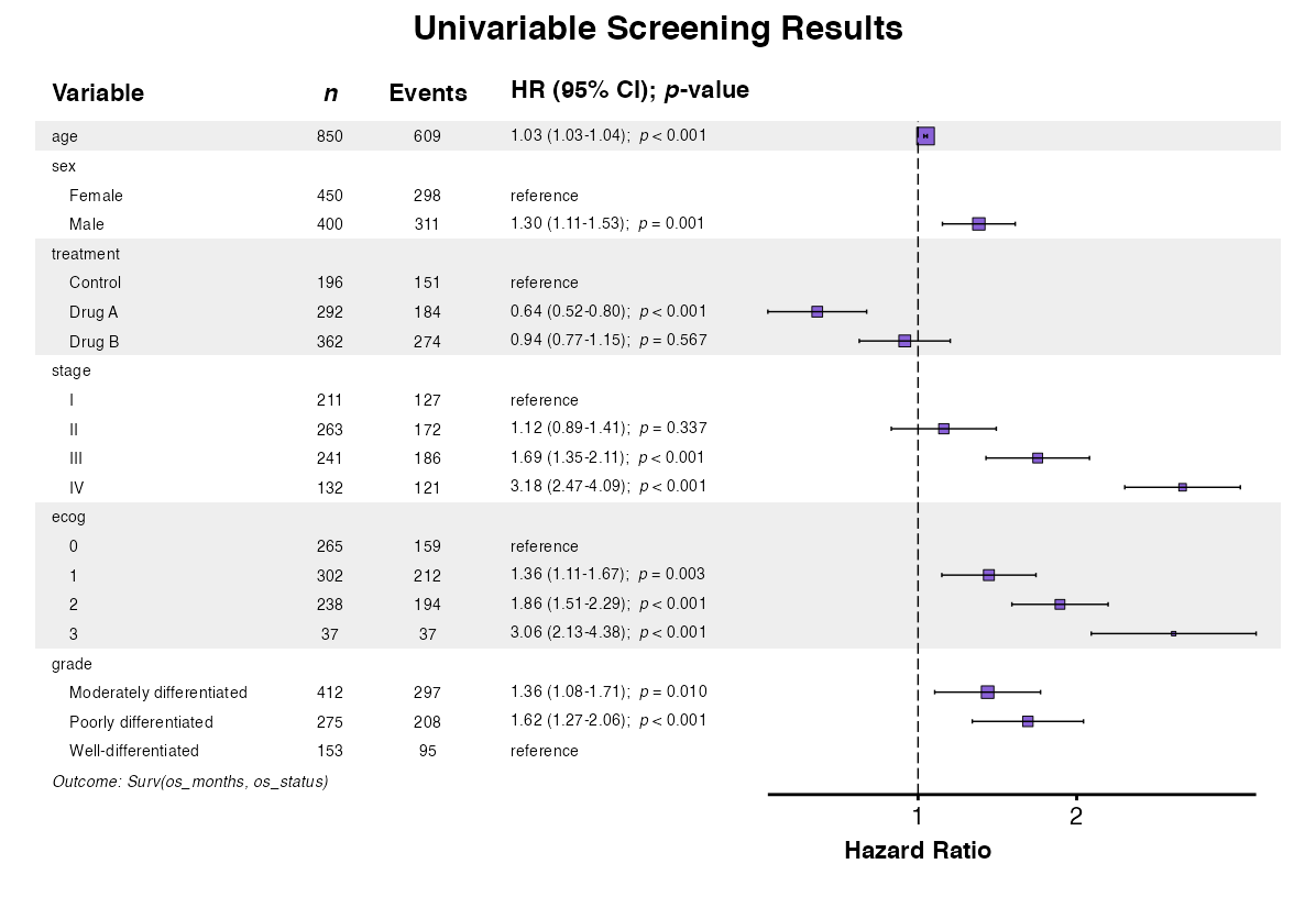

Advanced Multivariate Regression Features

The multifit() function supports interactions and mixed-effects models when testing a predictor across multiple outcomes.

Example 19: Multi-Outcome with Interactions

Test effect modification across multiple outcomes:

example19 <- multifit(
  data = clintrial,
  outcomes = c("surgery", "pfs_status", "os_status"),
  predictor = "treatment",
  covariates = c("age", "sex", "stage"),
  interactions = c("treatment:sex"),
  labels = clintrial_labels,
  parallel = FALSE
)

example19
##> 
##> Multivariate Analysis Results
##> Predictor: treatment
##> Outcomes: 3
##> Model Type: glm
##> Covariates: age, sex, stage
##> Interactions: treatment:sex
##> Display: adjusted
##> 
##>                        Outcome                             Predictor      n Events     aOR (95% CI) p-value
##>                         <char>                                <char> <char> <char>           <char>  <char>
##>  1:         Surgical Resection              Treatment Group (Drug A)    292    173 2.09 (1.20-3.62)   0.009
##>  2:         Surgical Resection              Treatment Group (Drug B)    361    102 0.50 (0.29-0.87)   0.013
##>  3:         Surgical Resection Treatment Group (Drug A) × Sex (Male)      -      - 0.77 (0.34-1.71)   0.515
##>  4:         Surgical Resection Treatment Group (Drug B) × Sex (Male)      -      - 0.79 (0.36-1.73)   0.554
##>  5: Progression or Death Event              Treatment Group (Drug A)    292    227 0.41 (0.20-0.84)   0.015
##>  6: Progression or Death Event              Treatment Group (Drug B)    361    321 0.95 (0.43-2.09)   0.893
##>  7: Progression or Death Event Treatment Group (Drug A) × Sex (Male)      -      - 0.75 (0.24-2.32)   0.618
##>  8: Progression or Death Event Treatment Group (Drug B) × Sex (Male)      -      - 0.63 (0.20-2.06)   0.448
##>  9:                Death Event              Treatment Group (Drug A)    292    184 0.39 (0.22-0.70)   0.002
##> 10:                Death Event              Treatment Group (Drug B)    361    273 0.61 (0.34-1.10)   0.099
##> 11:                Death Event Treatment Group (Drug A) × Sex (Male)      -      - 1.29 (0.53-3.18)   0.575
##> 12:                Death Event Treatment Group (Drug B) × Sex (Male)      -      - 1.59 (0.65-3.91)   0.308

Example 20: Multi-Outcome with Mixed Effects

Account for clustering when testing effects across outcomes:

example20 <- multifit(
  data = clintrial,
  outcomes = c("surgery", "pfs_status"),
  predictor = "treatment",
  covariates = c("age", "sex"),
  random = "(1|site)",
  model_type = "glmer",
  labels = clintrial_labels,
  parallel = FALSE
)

example20
##> 
##> Multivariate Analysis Results
##> Predictor: treatment
##> Outcomes: 2
##> Model Type: glmer
##> Covariates: age, sex
##> Random Effects: (1|site)
##> Display: adjusted
##> 
##>                       Outcome                Predictor      n Events     aOR (95% CI) p-value
##>                        <char>                   <char> <char> <char>           <char>  <char>
##> 1:         Surgical Resection Treatment Group (Drug A)    292    173 1.64 (1.13-2.40)   0.010
##> 2:         Surgical Resection Treatment Group (Drug B)    362    103 0.44 (0.30-0.63) < 0.001
##> 3: Progression or Death Event Treatment Group (Drug A)    292    227 0.41 (0.24-0.71)   0.001
##> 4: Progression or Death Event Treatment Group (Drug B)    362    322 1.01 (0.58-1.78)   0.971

Example 21: Survival Multi-Outcome with Mixed Effects

For multiple survival outcomes with clustering:

example21 <- multifit(
  data = clintrial,
  outcomes = c("Surv(pfs_months, pfs_status)",
               "Surv(os_months, os_status)"),
  predictor = "treatment",
  covariates = c("age", "sex"),
  random = "(1|site)",
  model_type = "coxme",
  labels = clintrial_labels,
  parallel = FALSE
)

example21
##> 
##> Multivariate Analysis Results
##> Predictor: treatment
##> Outcomes: 2
##> Model Type: coxme
##> Covariates: age, sex
##> Random Effects: (1|site)
##> Display: adjusted
##> 
##>                               Outcome                Predictor      n Events     aHR (95% CI) p-value
##>                                <char>                   <char> <char> <char>           <char>  <char>
##> 1: Progression-Free Survival (months) Treatment Group (Drug A)    723    723 0.63 (0.51-0.77) < 0.001
##> 2: Progression-Free Survival (months) Treatment Group (Drug B)    723    723 1.00 (0.83-1.20)   0.989
##> 3:          Overall Survival (months) Treatment Group (Drug A)    609    609 0.63 (0.50-0.78) < 0.001
##> 4:          Overall Survival (months) Treatment Group (Drug B)    609    609 1.00 (0.82-1.23)   0.962

Complete Workflow Example

The following demonstrates a complete advanced analysis workflow:

# Step 1: Screen risk factors for primary outcome
risk_screening <- uniscreen(
  data = clintrial,
  outcome = "os_status",
  predictors = c("age", "sex", "bmi", "smoking", "diabetes",
                 "hypertension", "stage", "ecog", "treatment"),
  model_type = "glm",
  p_threshold = 0.20,
  labels = clintrial_labels
)

risk_screening
##> 
##> Univariable Screening Results
##> Outcome: os_status
##> Model Type: Logistic
##> Predictors Screened: 9
##> Significant (p < 0.2): 6
##> 
##>                    Variable   Group      n Events            OR (95% CI) p-value
##>                      <char>  <char> <char> <char>                 <char>  <char>
##>  1:             Age (years)       -    850    609       1.05 (1.03-1.06) < 0.001
##>  2:                     Sex  Female    450    298              reference       -
##>  3:                            Male    400    311       1.78 (1.31-2.42) < 0.001
##>  4: Body Mass Index (kg/m²)       -    838    599       1.01 (0.98-1.05)   0.347
##>  5:          Smoking Status   Never    337    248              reference       -
##>  6:                          Former    311    203       0.67 (0.48-0.94)   0.022
##>  7:                         Current    185    143       1.22 (0.80-1.86)   0.351
##>  8:                Diabetes      No    637    457              reference       -
##>  9:                             Yes    197    138       0.92 (0.65-1.31)   0.646
##> 10:            Hypertension      No    504    354              reference       -
##> 11:                             Yes    331    242       1.15 (0.85-1.57)   0.369
##> 12:           Disease Stage       I    211    127              reference       -
##> 13:                              II    263    172       1.25 (0.86-1.82)   0.243
##> 14:                             III    241    186       2.24 (1.49-3.36) < 0.001
##> 15:                              IV    132    121      7.28 (3.70-14.30) < 0.001
##> 16: ECOG Performance Status       0    265    159              reference       -
##> 17:                               1    302    212       1.57 (1.11-2.22)   0.011
##> 18:                               2    238    194       2.94 (1.95-4.43) < 0.001
##> 19:                               3     37     37 10434240.53 (0.00-Inf)   0.967
##> 20:         Treatment Group Control    196    151              reference       -
##> 21:                          Drug A    292    184       0.51 (0.34-0.76)   0.001
##> 22:                          Drug B    362    274       0.93 (0.62-1.40)   0.721
##>                    Variable   Group      n Events            OR (95% CI) p-value
##>                      <char>  <char> <char> <char>                 <char>  <char>

# Step 2: Test key exposure across multiple outcomes
effects <- multifit(
  data = clintrial,
  outcomes = c("surgery", "pfs_status", "os_status"),
  predictor = "treatment",
  covariates = c("age", "sex", "stage"),
  columns = "both",
  labels = clintrial_labels,
  parallel = FALSE
)

effects
##> 
##> Multivariate Analysis Results
##> Predictor: treatment
##> Outcomes: 3
##> Model Type: glm
##> Covariates: age, sex, stage
##> Display: both
##> 
##>                       Outcome                Predictor      n Events      OR (95% CI)   Uni p     aOR (95% CI) Multi p
##>                        <char>                   <char> <char> <char>           <char>  <char>           <char>  <char>
##> 1:                Death Event Treatment Group (Drug A)    292    184 0.51 (0.34-0.76)   0.001 0.44 (0.28-0.68) < 0.001
##> 2:                Death Event Treatment Group (Drug B)    362    274 0.93 (0.62-1.40)   0.721 0.74 (0.48-1.16)   0.192
##> 3: Progression or Death Event Treatment Group (Drug A)    292    227 0.44 (0.26-0.74)   0.002 0.36 (0.21-0.63) < 0.001
##> 4: Progression or Death Event Treatment Group (Drug B)    362    322 1.02 (0.59-1.77)   0.950 0.77 (0.43-1.38)   0.374
##> 5:         Surgical Resection Treatment Group (Drug A)    292    173 1.58 (1.10-2.27)   0.014 1.84 (1.23-2.75)   0.003
##> 6:         Surgical Resection Treatment Group (Drug B)    362    103 0.43 (0.30-0.62) < 0.001 0.45 (0.30-0.66) < 0.001

# Step 3: Visualize effects
forest_plot <- multiforest(
  effects,
  title = "Effects Across Outcomes",
  indent_predictor = TRUE,
  zebra_stripes = TRUE
)
queue_plot(forest_plot)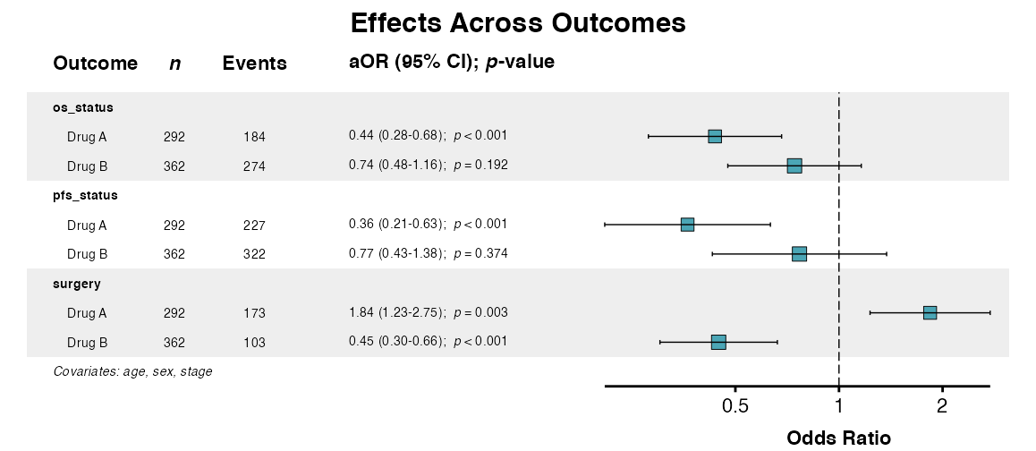

Best Practices

Interaction Analysis

Include main effects for all variables in interactions
Test formally using interaction p-values
Non-significant interactions do not prove effect homogeneity
Consider domain plausibility when interpreting

Mixed-Effects Models

Use when data exhibits natural clustering
Start with random intercepts; add random slopes if justified
Monitor convergence; simplify if necessary
Compare to fixed-effects models using compfit()

Method Selection

Scenario	Recommended Approach
Clustered observations	Mixed-effects models
Robust inference needed	Clustered standard errors
PH assumption violated	Stratification
Effect modification	Interaction terms
Survey data	Weighted regression

Sample Size Considerations

Interactions: Require larger samples than main effects models
Mixed models: Need sufficient clusters (≥ 20-30 recommended)
Stratification: Each stratum needs adequate events

Common Issues

Convergence Problems in Mixed Models

Simplify the random effects structure if convergence fails:

# Start with random intercepts only
fit(data, outcome, c(predictors, "(1|site)"), model_type = "lmer")

Check for common problems such as few observations per cluster, near-zero variance in random effects, or highly correlated predictors.

Interpreting Interactions

For categorical × categorical interactions, the coefficient represents the additional effect beyond the sum of main effects:

# Access model for detailed interpretation
model <- attr(result, "model")
summary(model)

Forest Plots with Interactions

Forest plots display all terms including interactions. For complex interaction patterns, consider stratified analyses or effect plots.

Preliminaries

Interaction Effects

Example 1: Two-Way Interaction

Example 2: Multiple Interactions

Example 3: Continuous × Categorical Interaction

Example 4: Interaction in fullfit()

Example 5: Testing Interaction Significance

Example 6: Forest Plot with Interactions

Mixed-Effects Models

Example 7: Random Intercepts (Linear Mixed)

Example 8: Random Intercepts (Logistic Mixed)

Example 9: Random Slopes

Example 10: Cox Mixed-Effects Model

Example 11: Forest Plot from Mixed Model

Example 12: Comparing Random-Effects Specifications

Stratification and Clustering

Example 13: Stratified Cox Model

Example 14: Cluster-Robust SEs

Weighted Regression

Example 15: Weighted Analysis

Advanced Univariable Screening Features

Example 16: Univariable Screening with Random Effects

Example 17: Cox Screening with Mixed Effects

Example 18: Forest Plot from Univariable Screening

Advanced Multivariate Regression Features

Example 19: Multi-Outcome with Interactions

Example 20: Multi-Outcome with Mixed Effects

Example 21: Survival Multi-Outcome with Mixed Effects

Complete Workflow Example

Best Practices

Interaction Analysis

Mixed-Effects Models

Method Selection

Sample Size Considerations

Common Issues

Convergence Problems in Mixed Models

Interpreting Interactions

Forest Plots with Interactions

Further Reading