Multivariate Regression

Multivariate regression refers to the simultaneous examination of a single independent predictor across multiple dependent variables. This approach inverts the typical regression paradigm: rather than testing multiple predictors against one outcome (as in uniscreen(), fit(), and fullfit()), multivariate regression tests the predictive value of a individual factor against multiple outcomes, with or without multivariable adjustment for other independent factors. This design is particularly useful when a key exposure or intervention must be evaluated against several endpoints simultaneously.

The multifit() function implements this workflow, supporting all model types available in summata with optional covariate adjustment, interaction terms, and mixed-effects specifications. Results can be visualized using multiforest() and exported using standard table export functions.

As with other summata functions, this function adheres to the standard calling convention:

multifit(data, outcomes, predictor, covariates, model_type, ...)

where data is the dataset, outcomes is a vector of screened outcome variables, predictor is the predicting variable under examination, covariates is a vector of simultaneous independent predicting variables (i.e., potential confounders), and model_type is the type of model to be implemented. This vignette demonstrates the various capabilities of this function using the included sample dataset.

Preliminaries

The examples in this vignette use the clintrial dataset included with summata:

library(summata)
library(survival)
library(ggplot2)

data(clintrial)
data(clintrial_labels)

The clintrial dataset includes multiple outcome types suitable for multivariate analysis:

Outcome Type	Variables	Model
Continuous	`los_days`, `pain_score`, `recovery_days`	`lm`
Binary	`any_complication`, `wound_infection`, `readmission_30d`, `icu_admission`	`glm` (binomial)
Count (equidispersed)	`fu_count`	`glm` (poisson)
Count (overdispersed)	`ae_count`	`negbin` or `quasipoisson`
Time-to-event	`Surv(pfs_months, pfs_status)`, `Surv(os_months, os_status)`	`coxph`

n.b.: To ensure correct font rendering and figure sizing, the forest plots below are displayed using a helper function (queue_plot()) that applies each plot’s recommended dimensions (stored in the "rec_dims" attribute) via the ragg graphics device. In practice, replace queue_plot() with ggplot2::ggsave() using recommended plot dimensions for equivalent results:
p <- glmforest(model, data = mydata)
dims <- attr(p, "rec_dims")
ggplot2::ggsave("forest_plot.png", p,
                width = dims$width, 
                height = dims$height)
This ensures that the figure size is always large enough to accommodate the constituent plot text and graphics, and it is generally the preferred method for saving forest plot outputs in summata.

Basic Usage

Example 1: Unadjusted Analysis

Test a single predictor against multiple binary outcomes:

example1 <- multifit(
  data = clintrial,
  outcomes = c("any_complication", "wound_infection",
               "readmission_30d", "icu_admission"),
  predictor = "surgery",
  labels = clintrial_labels,
  parallel = FALSE
)

example1
##> 
##> Multivariate Analysis Results
##> Predictor: surgery
##> Outcomes: 4
##> Model Type: glm
##> Display: unadjusted
##> 
##>                   Outcome          Predictor      n Events      OR (95% CI) p-value
##>                    <char>             <char> <char> <char>           <char>  <char>
##> 1:       Any Complication Surgical Resection    370    236 1.70 (1.29-2.25) < 0.001
##> 2:   Wound/Site Infection Surgical Resection    370    121 4.58 (3.16-6.66) < 0.001
##> 3:     30-Day Readmission Surgical Resection    370    181 0.91 (0.69-1.19)   0.500
##> 4: ICU Admission Required Surgical Resection    370    179 2.25 (1.70-2.99) < 0.001

Each row shows the effect of the predictor on a specific outcome. For categorical predictors, each non-reference level appears separately.

Example 2: Adjusted Analysis

Include covariates for confounding control:

example2 <- multifit(
  data = clintrial,
  outcomes = c("any_complication", "wound_infection",
               "readmission_30d", "icu_admission"),
  predictor = "surgery",
  covariates = c("age", "sex", "smoking", "diabetes"),
  labels = clintrial_labels,
  parallel = FALSE
)

example2
##> 
##> Multivariate Analysis Results
##> Predictor: surgery
##> Outcomes: 4
##> Model Type: glm
##> Covariates: age, sex, smoking, diabetes
##> Display: adjusted
##> 
##>                   Outcome          Predictor      n Events     aOR (95% CI) p-value
##>                    <char>             <char> <char> <char>           <char>  <char>
##> 1:       Any Complication Surgical Resection    362    229 1.84 (1.38-2.47) < 0.001
##> 2:   Wound/Site Infection Surgical Resection    362    117 5.21 (3.48-7.80) < 0.001
##> 3:     30-Day Readmission Surgical Resection    362    176 1.07 (0.80-1.43)   0.641
##> 4: ICU Admission Required Surgical Resection    362    173 2.56 (1.90-3.46) < 0.001

Example 3: Unadjusted and Adjusted Comparison

Use columns = "both" to display unadjusted and adjusted results side-by-side:

example3 <- multifit(
  data = clintrial,
  outcomes = c("any_complication", "wound_infection",
               "readmission_30d", "icu_admission"),
  predictor = "surgery",
  covariates = c("age", "sex", "diabetes", "surgery"),
  columns = "both",
  labels = clintrial_labels,
  parallel = FALSE
)

example3
##> 
##> Multivariate Analysis Results
##> Predictor: surgery
##> Outcomes: 4
##> Model Type: glm
##> Covariates: age, sex, diabetes, surgery
##> Display: both
##> 
##>                   Outcome          Predictor      n Events      OR (95% CI)   Uni p     aOR (95% CI) Multi p
##>                    <char>             <char> <char> <char>           <char>  <char>           <char>  <char>
##> 1:       Any Complication Surgical Resection    370    236 1.70 (1.29-2.25) < 0.001 1.82 (1.36-2.43) < 0.001
##> 2: ICU Admission Required Surgical Resection    370    179 2.25 (1.70-2.99) < 0.001 2.57 (1.90-3.47) < 0.001
##> 3:     30-Day Readmission Surgical Resection    370    181 0.91 (0.69-1.19)   0.500 1.05 (0.79-1.40)   0.720
##> 4:   Wound/Site Infection Surgical Resection    370    121 4.58 (3.16-6.66) < 0.001 4.98 (3.35-7.40) < 0.001

Comparing columns reveals confounding (large differences) or robust associations (similar estimates).

Predictor Types

Example 4: Continuous Predictors

For continuous predictors, one row appears per outcome:

example4 <- multifit(
  data = clintrial,
  outcomes = c("any_complication", "wound_infection", "icu_admission"),
  predictor = "age",
  covariates = c("sex", "treatment", "surgery"),
  labels = clintrial_labels,
  parallel = FALSE
)

example4
##> 
##> Multivariate Analysis Results
##> Predictor: age
##> Outcomes: 3
##> Model Type: glm
##> Covariates: sex, treatment, surgery
##> Display: adjusted
##> 
##>                   Outcome      n Events     aOR (95% CI) p-value
##>                    <char> <char> <char>           <char>  <char>
##> 1:       Any Complication    850    480 1.01 (1.00-1.03)   0.024
##> 2:   Wound/Site Infection    850    167 1.01 (0.99-1.02)   0.338
##> 3: ICU Admission Required    850    320 1.03 (1.02-1.04) < 0.001

The effect estimate represents the change in log-odds per one-unit increase in the predictor.

Example 5: Multilevel Categorical Predictors

For categorical predictors with multiple levels, the display is expanded:

example5 <- multifit(
  data = clintrial,
  outcomes = c("any_complication", "wound_infection",
               "readmission_30d", "icu_admission"),
  predictor = "treatment",
  covariates = c("age", "sex", "surgery"),
  labels = clintrial_labels,
  parallel = FALSE
)

example5
##> 
##> Multivariate Analysis Results
##> Predictor: treatment
##> Outcomes: 4
##> Model Type: glm
##> Covariates: age, sex, surgery
##> Display: adjusted
##> 
##>                   Outcome                Predictor      n Events     aOR (95% CI) p-value
##>                    <char>                   <char> <char> <char>           <char>  <char>
##> 1:       Any Complication Treatment Group (Drug A)    292    143 0.66 (0.45-0.96)   0.031
##> 2:       Any Complication Treatment Group (Drug B)    362    226 1.48 (1.03-2.14)   0.035
##> 3:   Wound/Site Infection Treatment Group (Drug A)    292     72 1.90 (1.14-3.17)   0.013
##> 4:   Wound/Site Infection Treatment Group (Drug B)    362     69 2.26 (1.34-3.79)   0.002
##> 5:     30-Day Readmission Treatment Group (Drug A)    292    127 0.86 (0.59-1.24)   0.415
##> 6:     30-Day Readmission Treatment Group (Drug B)    362    209 1.61 (1.12-2.31)   0.010
##> 7: ICU Admission Required Treatment Group (Drug A)    292    111 1.11 (0.74-1.65)   0.615
##> 8: ICU Admission Required Treatment Group (Drug B)    362    145 1.70 (1.16-2.50)   0.007

Model Types

Example 6: Cox Regression

For time-to-event outcomes, use model_type = "coxph":

example6 <- multifit(
  data = clintrial,
  outcomes = c("Surv(pfs_months, pfs_status)",
               "Surv(os_months, os_status)"),
  predictor = "treatment",
  covariates = c("age", "sex", "stage"),
  model_type = "coxph",
  labels = clintrial_labels,
  parallel = FALSE
)

example6
##> 
##> Multivariate Analysis Results
##> Predictor: treatment
##> Outcomes: 2
##> Model Type: coxph
##> Covariates: age, sex, stage
##> Display: adjusted
##> 
##>                               Outcome                Predictor      n Events     aHR (95% CI) p-value
##>                                <char>                   <char> <char> <char>           <char>  <char>
##> 1: Progression-Free Survival (months) Treatment Group (Drug A)    721    721 0.54 (0.44-0.66) < 0.001
##> 2: Progression-Free Survival (months) Treatment Group (Drug B)    721    721 0.82 (0.68-0.98)   0.033
##> 3:          Overall Survival (months) Treatment Group (Drug A)    606    606 0.56 (0.45-0.70) < 0.001
##> 4:          Overall Survival (months) Treatment Group (Drug B)    606    606 0.83 (0.67-1.01)   0.062

Example 7: Linear Regression

For continuous outcomes, use model_type = "lm":

example7 <- multifit(
  data = clintrial,
  outcomes = c("los_days", "pain_score", "recovery_days"),
  predictor = "treatment",
  covariates = c("age", "sex", "surgery"),
  model_type = "lm",
  labels = clintrial_labels,
  parallel = FALSE
)

example7
##> 
##> Multivariate Analysis Results
##> Predictor: treatment
##> Outcomes: 3
##> Model Type: lm
##> Covariates: age, sex, surgery
##> Display: adjusted
##> 
##>                            Outcome                Predictor      n Adj. Coefficient (95% CI) p-value
##>                             <char>                   <char> <char>                    <char>  <char>
##> 1:  Length of Hospital Stay (days) Treatment Group (Drug A)    288    -1.07 (-1.83 to -0.32)   0.006
##> 2:  Length of Hospital Stay (days) Treatment Group (Drug B)    350       3.10 (2.36 to 3.83) < 0.001
##> 3: Postoperative Pain Score (0-10) Treatment Group (Drug A)    289    -0.56 (-0.84 to -0.27) < 0.001
##> 4: Postoperative Pain Score (0-10) Treatment Group (Drug B)    359       0.86 (0.59 to 1.13) < 0.001
##> 5:     Days to Functional Recovery Treatment Group (Drug A)    288    -1.73 (-2.96 to -0.50)   0.006
##> 6:     Days to Functional Recovery Treatment Group (Drug B)    352       2.79 (1.60 to 3.98) < 0.001

Example 8: Mixed-Effects Models

Account for clustering using random effects:

example8 <- multifit(
  data = clintrial,
  outcomes = c("any_complication", "wound_infection"),
  predictor = "treatment",
  covariates = c("age", "sex"),
  random = "(1|site)",
  model_type = "glmer",
  labels = clintrial_labels,
  parallel = FALSE
)

example8
##> 
##> Multivariate Analysis Results
##> Predictor: treatment
##> Outcomes: 2
##> Model Type: glmer
##> Covariates: age, sex
##> Random Effects: (1|site)
##> Display: adjusted
##> 
##>                 Outcome                Predictor      n Events     aOR (95% CI) p-value
##>                  <char>                   <char> <char> <char>           <char>  <char>
##> 1:     Any Complication Treatment Group (Drug A)    292    143 0.74 (0.51-1.06)   0.104
##> 2:     Any Complication Treatment Group (Drug B)    362    226 1.29 (0.90-1.84)   0.170
##> 3: Wound/Site Infection Treatment Group (Drug A)    292     72 2.17 (1.32-3.57)   0.002
##> 4: Wound/Site Infection Treatment Group (Drug B)    362     69 1.62 (0.99-2.66)   0.055

Advanced Features

Example 9: Interaction Terms

Interaction terms can be added to test effect modification:

example9 <- multifit(
  data = clintrial,
  outcomes = c("any_complication", "wound_infection"),
  predictor = "treatment",
  covariates = c("age", "sex"),
  interactions = c("treatment:sex"),
  labels = clintrial_labels,
  parallel = FALSE
)

example9
##> 
##> Multivariate Analysis Results
##> Predictor: treatment
##> Outcomes: 2
##> Model Type: glm
##> Covariates: age, sex
##> Interactions: treatment:sex
##> Display: adjusted
##> 
##>                 Outcome                             Predictor      n Events     aOR (95% CI) p-value
##>                  <char>                                <char> <char> <char>           <char>  <char>
##> 1:     Any Complication              Treatment Group (Drug A)    292    143 0.63 (0.38-1.04)   0.074
##> 2:     Any Complication              Treatment Group (Drug B)    362    226 1.27 (0.78-2.08)   0.340
##> 3:     Any Complication Treatment Group (Drug A) × Sex (Male)      -      - 1.41 (0.68-2.93)   0.360
##> 4:     Any Complication Treatment Group (Drug B) × Sex (Male)      -      - 0.99 (0.48-2.00)   0.968
##> 5: Wound/Site Infection              Treatment Group (Drug A)    292     72 2.20 (1.13-4.28)   0.020
##> 6: Wound/Site Infection              Treatment Group (Drug B)    362     69 1.30 (0.66-2.57)   0.455
##> 7: Wound/Site Infection Treatment Group (Drug A) × Sex (Male)      -      - 0.93 (0.35-2.50)   0.884
##> 8: Wound/Site Infection Treatment Group (Drug B) × Sex (Male)      -      - 1.43 (0.54-3.83)   0.472

Example 10: Filtering by p-value

Outputs can be filtered to retain only significant associations:

example10 <- multifit(
  data = clintrial,
  outcomes = c("any_complication", "wound_infection",
               "readmission_30d", "icu_admission"),
  predictor = "treatment",
  covariates = c("age", "sex", "surgery"),
  p_threshold = 0.01,
  labels = clintrial_labels,
  parallel = FALSE
)

example10
##> 
##> Multivariate Analysis Results
##> Predictor: treatment
##> Outcomes: 4
##> Model Type: glm
##> Covariates: age, sex, surgery
##> Display: adjusted
##> 
##>                   Outcome                Predictor      n Events     aOR (95% CI) p-value
##>                    <char>                   <char> <char> <char>           <char>  <char>
##> 1:   Wound/Site Infection Treatment Group (Drug B)    362     69 2.26 (1.34-3.79)   0.002
##> 2:     30-Day Readmission Treatment Group (Drug B)    362    209 1.61 (1.12-2.31)   0.010
##> 3: ICU Admission Required Treatment Group (Drug B)    362    145 1.70 (1.16-2.50)   0.007

Example 11: Accessing Model Objects

Underlying model objects are stored as attributes for additional analysis:

result <- multifit(
  data = clintrial,
  outcomes = c("any_complication", "wound_infection"),
  predictor = "treatment",
  covariates = c("age", "sex"),
  labels = clintrial_labels,
  keep_models = TRUE,
  parallel = FALSE
)

# Access individual models
models <- attr(result, "models")
names(models)
##> [1] "any_complication" "wound_infection"

# Examine a specific model
summary(models[["any_complication"]])
##>          Length Class Mode
##> adjusted 30     glm   list

Forest Plot Visualization

The multiforest() function creates forest plots from multifit() results.

Example 12: Forest Plot for Logistic (Binary) Outcomes

Results from multifit() can be directly inserted into the multiforest() function to generate a forest plot:

result <- multifit(
  data = clintrial,
  outcomes = c("any_complication", "wound_infection",
               "readmission_30d", "icu_admission"),
  predictor = "treatment",
  covariates = c("age", "sex", "diabetes", "surgery"),
  labels = clintrial_labels,
  parallel = FALSE
)

example12 <- multiforest(
  result,
  title = "Treatment Effects Across Outcomes",
  indent_predictor = TRUE,
  zebra_stripes = TRUE
)
queue_plot(example12)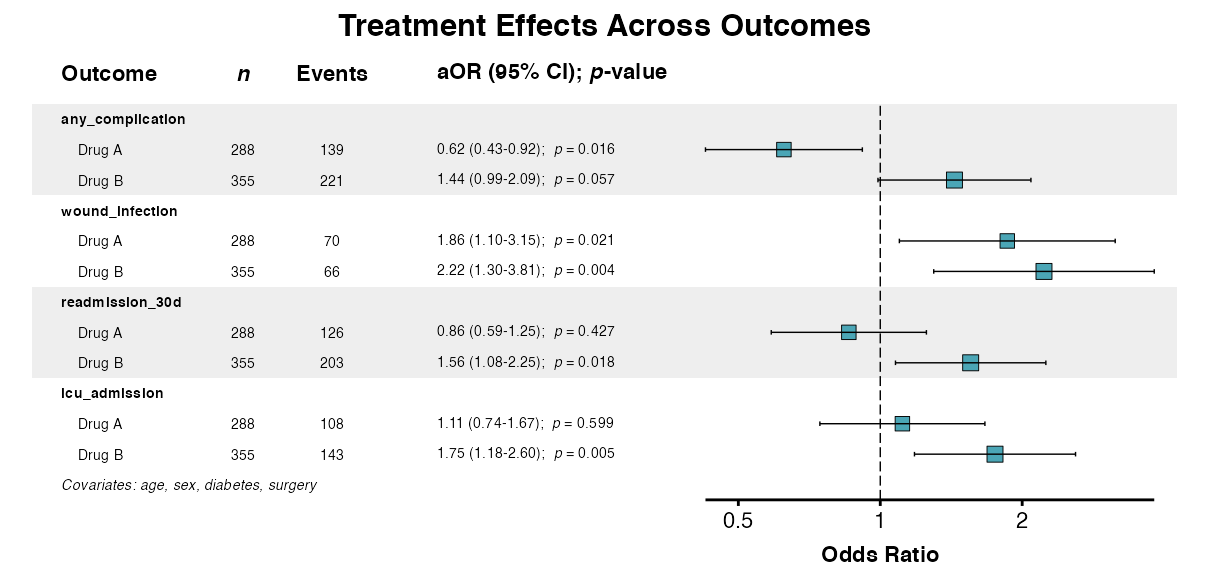

Example 13: Customization Options

Customize the appearance of the forest plot by adjusting function parameters:

example13 <- multiforest(
  result,
  title = "Effect Estimates",
  column = "adjusted",
  show_predictor = FALSE,
  covariates_footer = TRUE,
  table_width = 0.65,
  color = "#4BA6B6"
)
queue_plot(example13)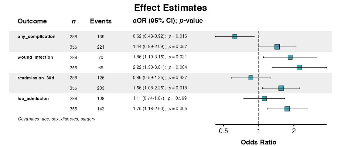

Example 14: Forest Plot for Continuous Outcomes

Create forest plots for continuous outcomes:

lm_result <- multifit(
  data = clintrial,
  outcomes = c("pain_score", "recovery_days", "los_days"),
  predictor = "treatment",
  covariates = c("age", "sex", "surgery"),
  model_type = "lm",
  parallel = FALSE
)

example14 <- multiforest(
  lm_result,
  title = "Treatment Effects on Recovery Metrics",
  show_predictor = FALSE,
  covariates_footer = TRUE,
  labels = clintrial_labels
)
queue_plot(example14)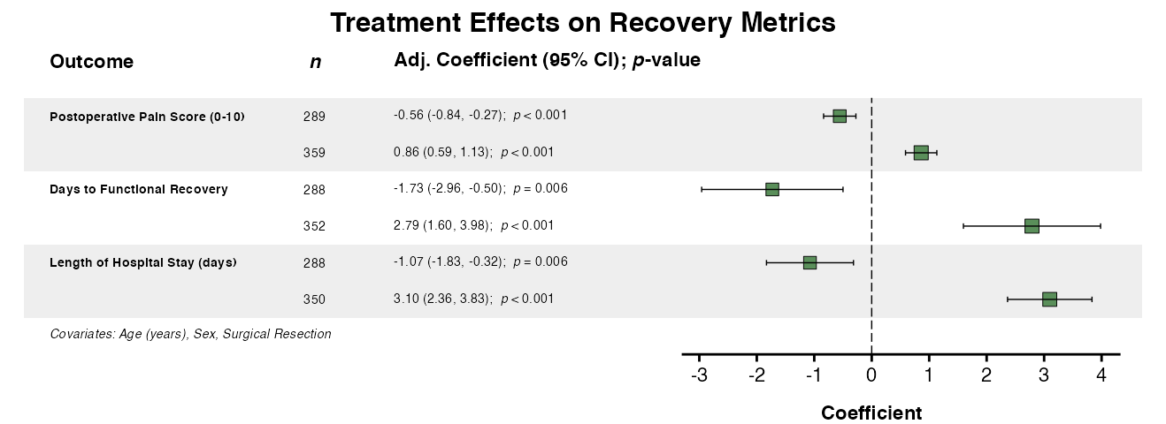

Example 15: Forest Plot for Survival Outcomes

The multiforest() function supports multiple model_type outputs from multifit(). In addition, variable labels can be applied to multiforest() outputs similarly to other forest plot functions:

cox_result <- multifit(
  data = clintrial,
  outcomes = c("Surv(pfs_months, pfs_status)",
               "Surv(os_months, os_status)"),
  predictor = "treatment",
  covariates = c("age", "sex", "stage"),
  model_type = "coxph",
  parallel = FALSE
)

example15 <- multiforest(
  cox_result,
  title = "Treatment Effects on Survival Outcomes",
  indent_predictor = TRUE,
  zebra_stripes = TRUE,
  labels = clintrial_labels
)
queue_plot(example15)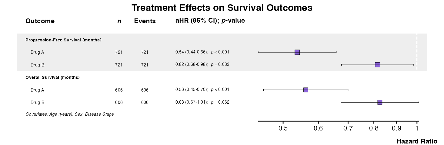

Exporting Results

Tables

Export tables using standard export functions:

table2docx(
  table = result,
  file = file.path(tempdir(), "multioutcome_analysis.docx"),
  caption = "Treatment Effects Across Outcomes"
)

table2pdf(
  table = result,
  file = file.path(tempdir(), "multioutcome_analysis.pdf"),
  caption = "Treatment Effects Across Outcomes"
)

Forest Plots

Save forest plots using ggsave():

p <- multiforest(result, title = "Effect Estimates")
dims <- attr(p, "rec_dims")

ggsave(file.path(tempdir(), "multioutcome_forest.pdf"), p,
       width = attr(result, "rec_dims")$width,
       height = attr(result, "rec_dims")$height, 
       units = "in")

Complete Workflow Example

The following demonstrates a complete multi-outcome analysis workflow:

## Define outcomes by type
binary_outcomes <- c("any_complication", "wound_infection",
                     "readmission_30d", "icu_admission")
survival_outcomes <- c("Surv(pfs_months, pfs_status)",
                       "Surv(os_months, os_status)")

## Unadjusted screening
unadjusted <- multifit(
  data = clintrial,
  outcomes = binary_outcomes,
  predictor = "treatment",
  labels = clintrial_labels,
  parallel = FALSE
)

unadjusted
##> 
##> Multivariate Analysis Results
##> Predictor: treatment
##> Outcomes: 4
##> Model Type: glm
##> Display: unadjusted
##> 
##>                   Outcome                Predictor      n Events      OR (95% CI) p-value
##>                    <char>                   <char> <char> <char>           <char>  <char>
##> 1:       Any Complication Treatment Group (Drug A)    292    143 0.73 (0.51-1.06)   0.097
##> 2:       Any Complication Treatment Group (Drug B)    362    226 1.27 (0.89-1.81)   0.182
##> 3:   Wound/Site Infection Treatment Group (Drug A)    292     72 2.14 (1.31-3.50)   0.002
##> 4:   Wound/Site Infection Treatment Group (Drug B)    362     69 1.54 (0.94-2.51)   0.084
##> 5:     30-Day Readmission Treatment Group (Drug A)    292    127 0.89 (0.62-1.28)   0.523
##> 6:     30-Day Readmission Treatment Group (Drug B)    362    209 1.58 (1.11-2.24)   0.011
##> 7: ICU Admission Required Treatment Group (Drug A)    292    111 1.26 (0.86-1.85)   0.226
##> 8: ICU Admission Required Treatment Group (Drug B)    362    145 1.38 (0.96-1.99)   0.085

## Adjusted analysis with comparison
adjusted <- multifit(
  data = clintrial,
  outcomes = binary_outcomes,
  predictor = "treatment",
  covariates = c("age", "sex", "diabetes", "surgery"),
  columns = "both",
  labels = clintrial_labels,
  parallel = FALSE
)

adjusted
##> 
##> Multivariate Analysis Results
##> Predictor: treatment
##> Outcomes: 4
##> Model Type: glm
##> Covariates: age, sex, diabetes, surgery
##> Display: both
##> 
##>                   Outcome                Predictor      n Events      OR (95% CI)  Uni p     aOR (95% CI) Multi p
##>                    <char>                   <char> <char> <char>           <char> <char>           <char>  <char>
##> 1:       Any Complication Treatment Group (Drug A)    292    143 0.73 (0.51-1.06)  0.097 0.62 (0.43-0.92)   0.016
##> 2:       Any Complication Treatment Group (Drug B)    362    226 1.27 (0.89-1.81)  0.182 1.44 (0.99-2.09)   0.057
##> 3: ICU Admission Required Treatment Group (Drug A)    292    111 1.26 (0.86-1.85)  0.226 1.11 (0.74-1.67)   0.599
##> 4: ICU Admission Required Treatment Group (Drug B)    362    145 1.38 (0.96-1.99)  0.085 1.75 (1.18-2.60)   0.005
##> 5:     30-Day Readmission Treatment Group (Drug A)    292    127 0.89 (0.62-1.28)  0.523 0.86 (0.59-1.25)   0.427
##> 6:     30-Day Readmission Treatment Group (Drug B)    362    209 1.58 (1.11-2.24)  0.011 1.56 (1.08-2.25)   0.018
##> 7:   Wound/Site Infection Treatment Group (Drug A)    292     72 2.14 (1.31-3.50)  0.002 1.86 (1.10-3.15)   0.021
##> 8:   Wound/Site Infection Treatment Group (Drug B)    362     69 1.54 (0.94-2.51)  0.084 2.22 (1.30-3.81)   0.004

## Forest plot visualization
forest_plot <- multiforest(
  adjusted,
  title = "Treatment Effect Estimates",
  column = "adjusted",
  indent_predictor = TRUE,
  zebra_stripes = TRUE,
  table_width = 0.65,
  labels = clintrial_labels
)
queue_plot(forest_plot)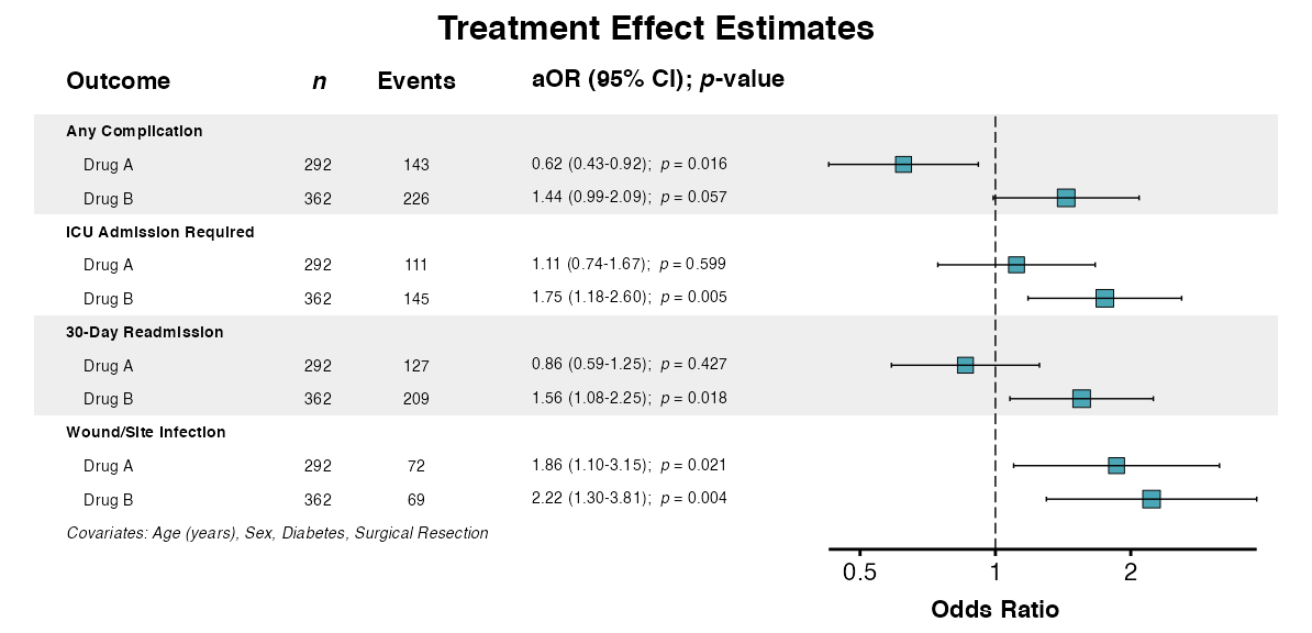

Parameter Reference

Parameter	Description
`outcomes`	Character vector of outcome variable names
`predictor`	Single predictor variable name
`covariates`	Optional adjustment covariates
`interactions`	Interaction terms (colon notation)
`random`	Random effects formula for mixed models
`strata`	Stratification variable (Cox models)
`cluster`	Clustering variable for robust standard errors
`model_type`	`"glm"`, `"lm"`, `"coxph"`, `"glmer"`, `"lmer"`, `"coxme"`
`family`	GLM family (default: `"binomial"`)
`columns`	`"adjusted"`, `"unadjusted"`, or `"both"`
`p_threshold`	Filter results by p-value
`labels`	Custom variable labels
`parallel`	Enable parallel processing

Best Practices

Outcome Selection

Use compatible outcome types within a single analysis
Group conceptually related outcomes
Consider multiple testing adjustments when testing many outcomes

Adjustment Strategy

Pre-specify covariates based on domain knowledge
Use columns = "both" to assess confounding
Apply consistent covariates across outcomes for comparability

Interpretation

Focus on effect magnitude and precision, not only p-values
Look for consistent patterns across related outcomes
Consider practical significance alongside statistical significance

Common Issues

Empty Results

If results are empty, verify:

Predictor variable exists and has variation
Outcomes are correctly specified (Surv() syntax for survival)
Model type matches outcome type

Convergence Warnings

For mixed-effects models, simplify the random effects structure:

## Start with random intercepts only
multifit(data, outcomes, predictor,
         random = "(1|site)",
         model_type = "glmer")

Many Factor Levels

For predictors with many levels, consider collapsing categories:

clintrial$treatment_binary <- ifelse(clintrial$treatment == "Control", 
                                      "Control", "Active")

Other Considerations

Multivariate Regression vs. Univariable Screening

The distinction between multifit() and uniscreen() is important:

Function	Tests	Use Case
`uniscreen()`	Multiple predictors → One outcome	Variable screening, risk factor identification
`multifit()`	One predictor → Multiple outcomes	Exposure effects, intervention evaluation

All outcomes in a single multifit() call should be of the same type (all binary, all continuous, or all survival). Mixing outcome types produces tables with incompatible effect measures. The function validates outcome compatibility and issues a warning when mixed types are detected.

Categorical Outcomes with More Than Two Levels

multifit() supports binary outcomes (via logistic regression) but not multinomial or ordinal outcomes. If a categorical outcome with three or more levels is included (e.g., treatment group with “Control”, “Drug A”, “Drug B”), the function will issue a warning because binomial GLM coerces such variables to binary (first level vs. all others).

For multilevel categorical outcomes, use dedicated packages outside of summata:

## Multinomial regression (unordered categories)
library(nnet)
model <- multinom(treatment ~ age + sex + stage, data = clintrial)

## Ordinal regression (ordered categories)
library(MASS)
model <- polr(grade ~ age + sex + stage, data = clintrial, Hess = TRUE)