Execution speed is rarely the primary consideration when selecting statistical software—correctness, interpretability, and ease-of-use usually take precedence. However, computational efficiency becomes relevant when working with large datasets, conducting simulation studies, or iterating through model specifications during exploratory analysis.
This article documents the computational performance of
summata relative to established alternatives. The
benchmarks presented here are intended as a reference for users whose
workflows involve performance-sensitive operations, and as a record of
the design tradeoffs inherent in different implementation
approaches.
Methodology
All benchmarks were conducted using the microbenchmark
package under the following conditions:
- Iterations: 5–20 per benchmark, adjusted for computational intensity
- Dataset sizes: 500 to 10,000 observations
- Data structure: Simulated clinical trial data with continuous, categorical, and time-to-event variables
- Predictors: 14 variables for screening benchmarks
Datasets were generated using a fixed random seed to ensure reproducibility. Timing measurements exclude package loading and data generation. All packages were tested using default parameters unless otherwise noted.
Two summata configurations are benchmarked throughout:
the default configuration, which uses profile
likelihood confidence intervals for GLM models and includes full
formatting (QC statistics, sample sizes, reference rows); and a
minimal configuration (summata_minimal),
which uses Wald CIs and disables optional output features. This
distinction is important because profile likelihood CIs dominate GLM
execution time, and the minimal configuration provides a way to measure
summata’s formatting overhead in isolation. Note that
finalfit and broom also use profile likelihood
CIs by default for GLM models.
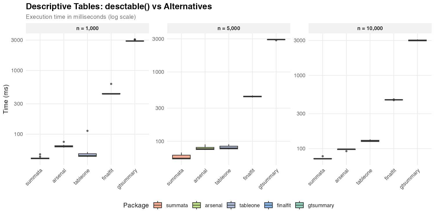
Descriptive Tables
Descriptive summary tables represent a common first step in data analysis. The following packages provide comparable functionality with differing implementation strategies.
| Package | Function | Implementation Notes |
|---|---|---|
summata |
desctable() |
data.table operations |
arsenal |
tableby() |
Formula-based interface |
tableone |
CreateTableOne() |
Matrix-based computation |
finalfit |
summary_factorlist() |
tidyverse ecosystem |
gtsummary |
tbl_summary() |
gt table framework |
| Dataset Size | summata |
arsenal |
tableone |
finalfit |
gtsummary |
|---|---|---|---|---|---|
| n = 1,000 | 42 ms | 64 ms | 46 ms | 429 ms | 2,901 ms |
| n = 5,000 | 57 ms | 77 ms | 79 ms | 442 ms | 2,929 ms |
| n = 10,000 | 73 ms | 98 ms | 126 ms | 464 ms | 3,001 ms |
The observed timing differences reflect underlying implementation
choices. Packages built on data.table or base R matrix
operations (summata, tableone,
arsenal) exhibit lower overhead than those employing more
extensive formatting pipelines (gtsummary). The
gtsummary package prioritizes output flexibility and
gt integration, which introduces additional computational
cost.
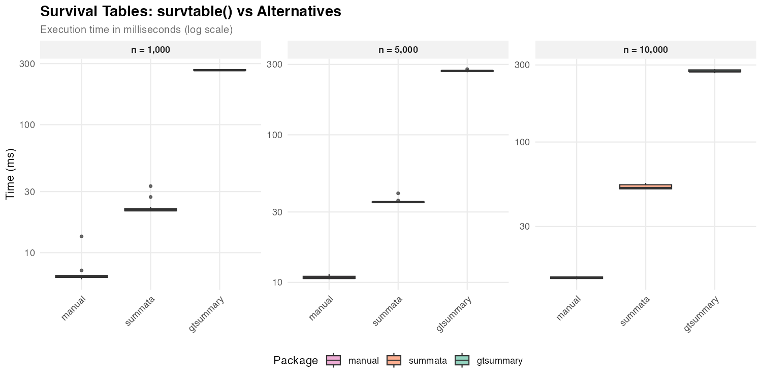
Survival Tables
Survival probability tables summarize Kaplan-Meier estimates at specified time points.
| Package | Function | Notes |
|---|---|---|
summata |
survtable() |
Formatted output |
| manual | survival::survfit() |
Raw computation |
gtsummary |
tbl_survfit() |
gt integration |
| Dataset Size | summata |
gtsummary |
manual |
|---|---|---|---|
| n = 1,000 | 21 ms | 266 ms | 6 ms |
| n = 5,000 | 35 ms | 271 ms | 11 ms |
| n = 10,000 | 52 ms | 274 ms | 14 ms |
Direct survfit() computation provides a baseline for the
minimum time required. The difference between raw computation and
formatted output reflects the cost of table construction and
presentation logic.
Regression Output
The following benchmarks compare functions that extract and format regression coefficients. Each package produces tables suitable for publication, though with varying levels of default formatting. Compared functions are as follows:
| Package | Function | Notes |
|---|---|---|
summata |
fit() |
Profile likelihood CIs, QC stats, counts, and reference rows |
summata_minimal |
fit(..., conf_method = "wald", show_n = FALSE, show_events = FALSE, reference_rows = FALSE, keep_qc_stats = FALSE) |
Wald CIs, reduced output |
finalfit |
glmuni() + fit2df()
|
Profile likelihood CIs (default) |
broom |
tidy() |
Profile likelihood CIs via confint()
dispatch |
gtsummary |
tbl_regression() |
gt formatting |
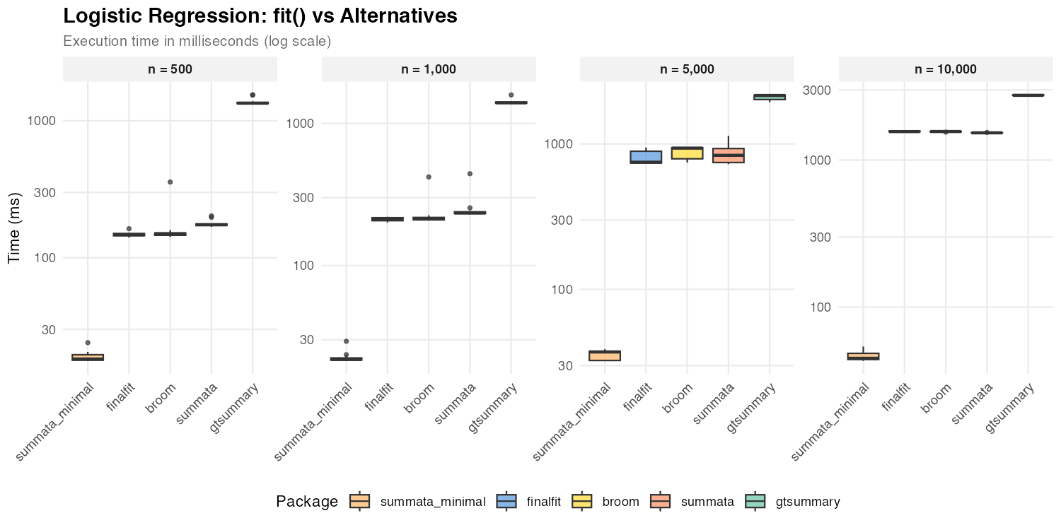
Logistic Regression
| Dataset Size | summata_minimal |
summata |
finalfit |
broom |
gtsummary |
|---|---|---|---|---|---|
| n = 500 | 18 ms | 174 ms | 147 ms | 150 ms | 1,344 ms |
| n = 1,000 | 22 ms | 234 ms | 212 ms | 214 ms | 1,399 ms |
| n = 5,000 | 37 ms | 840 ms | 749 ms | 936 ms | 2,153 ms |
| n = 10,000 | 45 ms | 1,532 ms | 1,562 ms | 1,564 ms | 2,756 ms |
The default summata configuration uses profile
likelihood confidence intervals for GLM models, as do
finalfit and broom::tidy(). The three packages
show comparable performance for logistic regression because profile
likelihood profiling dominates execution time for all of them. The
summata_minimal configuration uses Wald CIs instead,
skipping the profiling step entirely, and achieves the fastest
extraction times at all sample sizes. At large n, profiling
cost grows with the number of IRLS iterations, causing all profile-based
packages to converge toward similar timings.
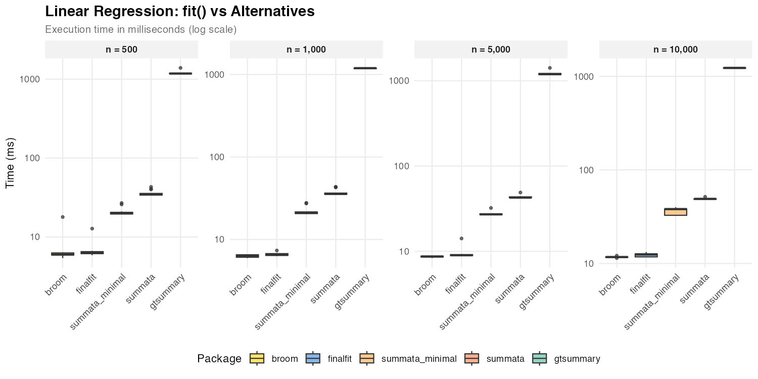
Linear Regression
| Dataset Size | summata_minimal |
summata |
finalfit |
broom |
gtsummary |
|---|---|---|---|---|---|
| n = 500 | 20 ms | 35 ms | 6 ms | 6 ms | 1,179 ms |
| n = 1,000 | 21 ms | 36 ms | 7 ms | 6 ms | 1,193 ms |
| n = 5,000 | 27 ms | 43 ms | 9 ms | 9 ms | 1,192 ms |
| n = 10,000 | 38 ms | 49 ms | 13 ms | 12 ms | 1,230 ms |
For linear models, broom::tidy() and
finalfit achieve faster coefficient extraction due to lower
formatting overhead. All three packages use exact
t-distribution CIs for lm objects (via
confint.lm()), so the timing difference reflects formatting
features (reference rows, QC statistics) rather than CI computation.
Poisson Regression
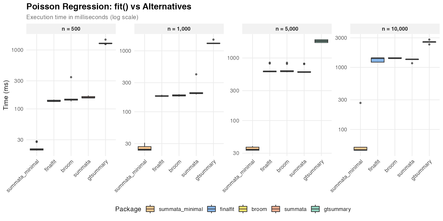
| Dataset Size | summata_minimal |
summata |
finalfit |
broom |
gtsummary |
|---|---|---|---|---|---|
| n = 500 | 20 ms | 155 ms | 135 ms | 144 ms | 1,293 ms |
| n = 1,000 | 24 ms | 201 ms | 181 ms | 184 ms | 1,325 ms |
| n = 5,000 | 34 ms | 595 ms | 613 ms | 612 ms | 1,868 ms |
| n = 10,000 | 47 ms | 1,351 ms | 1,409 ms | 1,402 ms | 2,577 ms |
Poisson regression shows the same profile likelihood pattern as
logistic regression: the default summata,
finalfit, and broom all use profile CIs and
show comparable performance. The summata_minimal
configuration with Wald CIs is consistently the fastest option.
Cox Regression
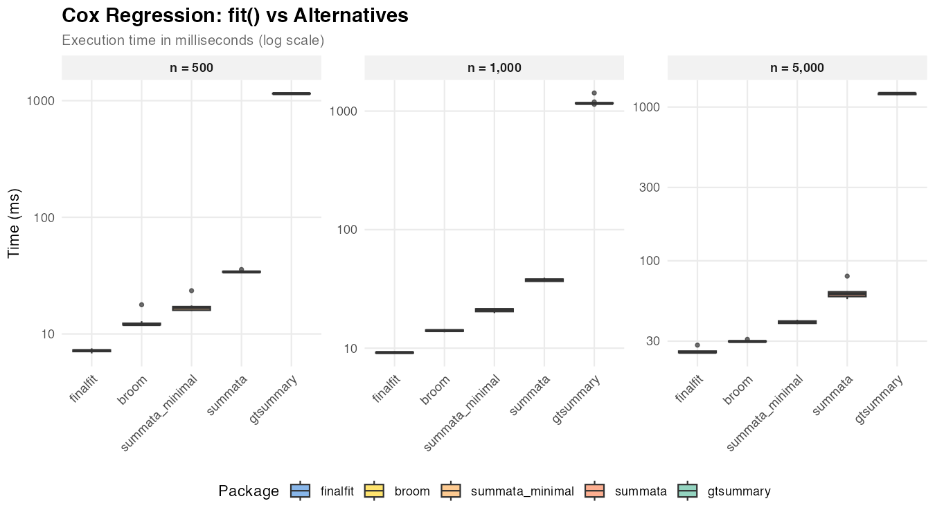
| Dataset Size | summata_minimal | summata | finalfit | broom | gtsummary |
|---|---|---|---|---|---|
| n = 500 | 17 ms | 34 ms | 7 ms | 12 ms | 1,149 ms |
| n = 1,000 | 21 ms | 38 ms | 9 ms | 14 ms | 1,161 ms |
| n = 5,000 | 40 ms | 61 ms | 25 ms | 30 ms | 1,227 ms |
Cox models use Wald CIs regardless of the conf_method
setting (the standard approach in survival analysis), so the timing
difference between summata and summata_minimal
reflects formatting overhead only. finalfit and
broom achieve faster extraction with less formatting.
Mixed-Effects Models
Mixed-effects models present a useful comparison case because the
underlying model fitting (via lme4) dominates execution
time regardless of the wrapper package.
| Package | Function | Notes |
|---|---|---|
summata |
fit(..., model_type = "lmer") |
Unified interface |
summata_minimal |
fit(..., model_type = "lmer", conf_method = "wald", show_n = FALSE, show_events = FALSE, reference_rows = FALSE, keep_qc_stats = FALSE) |
Reduced output |
finalfit |
lmmixed() + fit2df()
|
Two-step process |
broom.mixed |
tidy() |
Minimal extraction |
gtsummary |
tbl_regression() |
gt formatting |
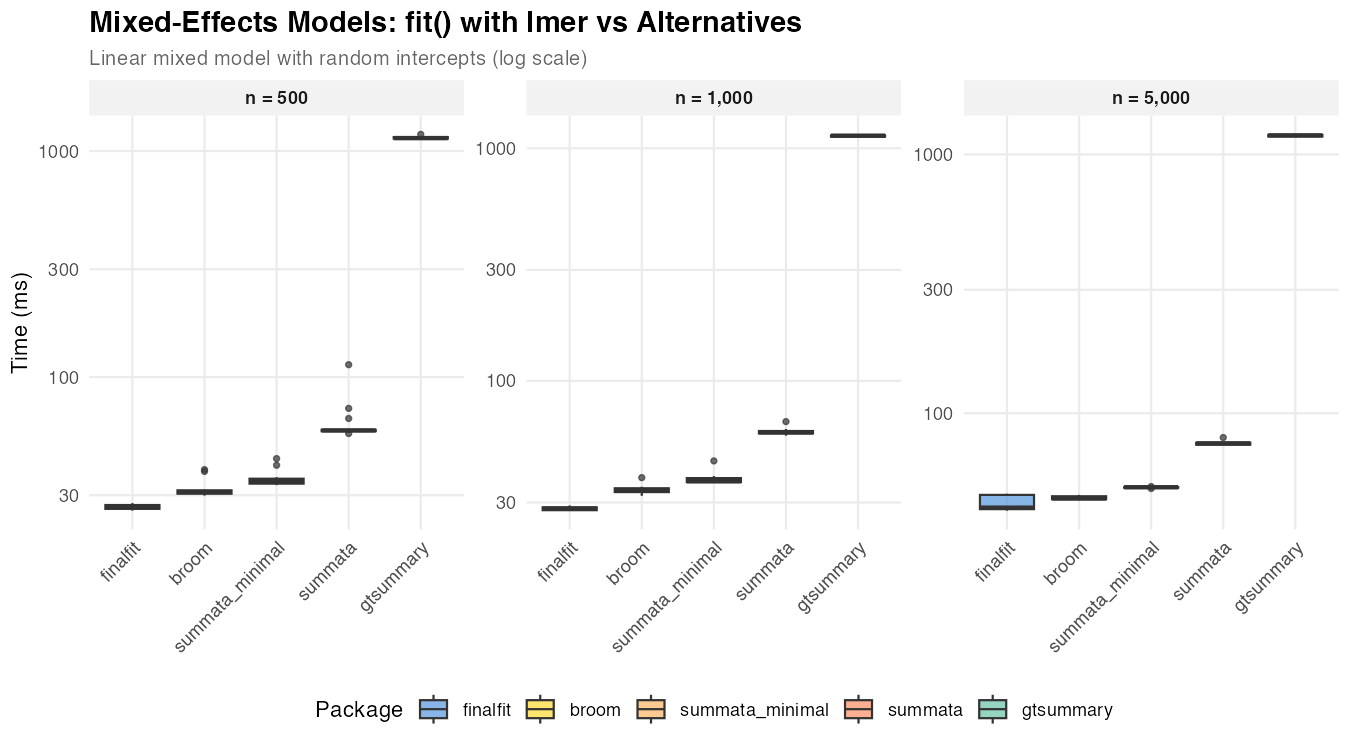
| Dataset Size | summata_minimal |
summata |
finalfit |
broom |
gtsummary |
|---|---|---|---|---|---|
| n = 500 | 35 ms | 58 ms | 26 ms | 31 ms | 1,141 ms |
| n = 1,000 | 37 ms | 60 ms | 28 ms | 34 ms | 1,133 ms |
| n = 5,000 | 52 ms | 76 ms | 43 ms | 47 ms | 1,185 ms |
The relatively narrow spread among summata,
finalfit, and broom reflects the dominance of
model fitting time. Differences in wrapper overhead become
proportionally less significant as the underlying computation grows.
Univariable Screening
Univariable screening—fitting separate models for each predictor—provides a test case for operations involving many repeated model fits.
| Package | Function | Notes |
|---|---|---|
summata |
uniscreen() |
Parallel-capable |
summata_minimal |
uniscreen(..., conf_method = "wald", show_n = FALSE, show_events = FALSE, reference_rows = FALSE) |
Wald CIs, reduced output |
finalfit |
glmuni() + fit2df()
|
Sequential |
broom |
Loop + tidy()
|
Manual implementation |
arsenal |
modelsum() |
Formula interface |
gtsummary |
tbl_uvregression() |
gt formatting |
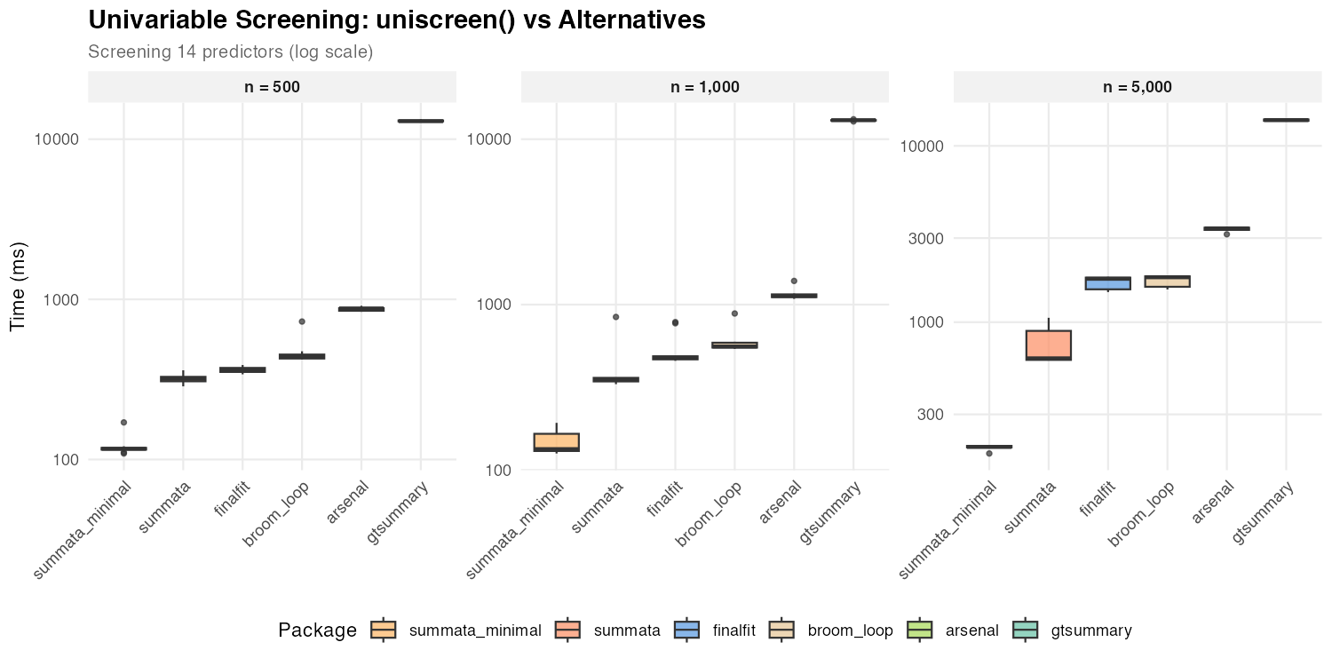
Screening 14 predictors:
| Dataset Size | summata_minimal |
summata |
finalfit |
broom |
arsenal |
gtsummary |
|---|---|---|---|---|---|---|
| n = 500 | 117 ms | 319 ms | 360 ms | 440 ms | 877 ms | 12,963 ms |
| n = 1,000 | 134 ms | 351 ms | 477 ms | 558 ms | 1,128 ms | 13,025 ms |
| n = 5,000 | 196 ms | 624 ms | 1,763 ms | 1,799 ms | 3,401 ms | 14,001 ms |
The performance gap between summata (default) and
summata_minimal is amplified during univariable screening
because profile likelihood profiling is repeated for each of the 14
predictor models. All profile-based packages (summata
default, finalfit, broom) show comparable
performance, as profiling dominates their execution time. With Wald CIs,
summata_minimal is the fastest option at all sample sizes,
outperforming the next-fastest alternative by 2.6–9.0× due to
data.table vectorization and parallel model fitting.
Complete Workflow
The combined univariable screening and multivariable modeling workflow represents a common analytical pattern in statistical research.
| Package | Approach | Notes |
|---|---|---|
summata |
fullfit() |
Single function |
summata_minimal |
fullfit(..., conf_method = "wald", show_n = FALSE, show_events = FALSE, reference_rows = FALSE) |
Wald CIs, reduced output |
finalfit |
finalfit() |
Single function |
| manual | Loop + glm() + broom::tidy()
+ rbind()
|
Custom |
gtsummary |
tbl_uvregression() +
tbl_regression() + tbl_merge()
|
Multi-step |
| Dataset Size | summata_minimal |
summata |
finalfit |
manual | gtsummary |
|---|---|---|---|---|---|
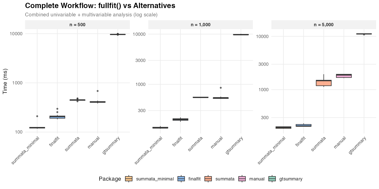
| n = 500 | 123 ms | 450 ms | 207 ms | 407 ms | 9,655 ms |
| n = 1,000 | 136 ms | 549 ms | 200 ms | 541 ms | 9,726 ms |
| n = 5,000 | 196 ms | 1,479 ms | 209 ms | 1,889 ms | 11,092 ms |
The default summata and finalfit show
comparable performance for GLM workflows because both use profile
likelihood CIs. The difference between them reflects
summata’s additional features (QC statistics, reference
rows, complete-case sample sizes) versus finalfit’s
inclusion of a descriptive statistics table. The
summata_minimal configuration with Wald CIs is the fastest
single-function option at small to moderate sample sizes, completing the
combined analysis in roughly 60–70% of the time finalfit
requires at n = 500–1,000.
Forest Plots
Forest plot generation combines data extraction with graphical rendering.
| Package | Function | Notes |
|---|---|---|
summata |
coxforest() |
Integrated table and plot |
survminer |
ggforest() |
Survival-focused |
| manual | Custom ggplot2
|
Maximum flexibility |
| Dataset Size | summata |
survminer |
manual |
|---|---|---|---|
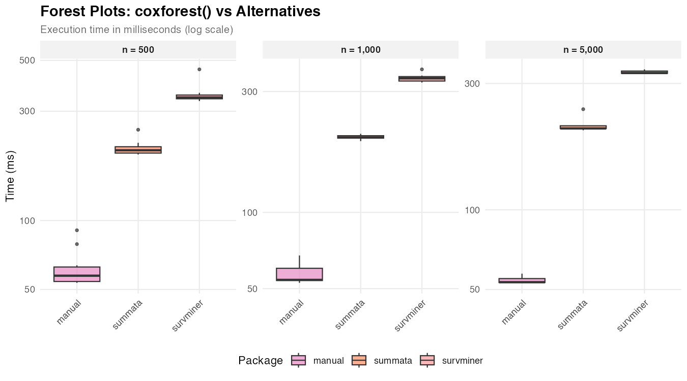
| n = 500 | 203 ms | 345 ms | 57 ms |
| n = 1,000 | 198 ms | 338 ms | 54 ms |
| n = 5,000 | 203 ms | 329 ms | 53 ms |
The manual approach produces only the graphical element, while
summata and survminer generate integrated
displays with coefficient tables. The relatively constant timing across
dataset sizes indicates that plot rendering, rather than data
processing, dominates execution time. Also, there are significant
cosmetic differences between the three graphical outputs, which
predominates other factors when selecting a plotting function.
Relative Performance
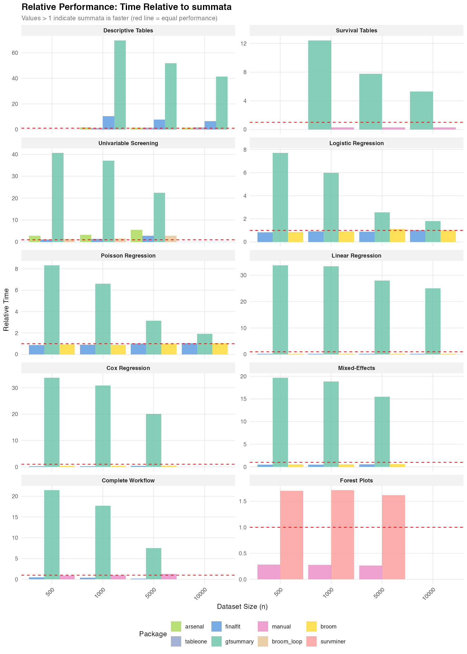
The following figures summarize timing ratios across benchmarks. Values greater than 1 indicate the comparison package requires more time than the baseline.
Summary of Ratios
Ratios relative to summata (default):
| Benchmark | gtsummary |
finalfit |
arsenal |
|---|---|---|---|
| Descriptive Tables | 41–70× | 6–10× | 1.4–1.5× |
| Survival Tables | 5–12× | — | — |
| Logistic Regression | 6–8× | 0.8–1.0× | — |
| Poisson Regression | 7–8× | 0.9–1.0× | — |
| Linear Regression | 25–34× | 0.2–0.3× | — |
| Cox Regression | 20–34× | 0.2–0.4× | — |
| Mixed-Effects | 16–20× | 0.5–0.6× | — |
| Univariable Screening | 22–41× | 1.1–2.8× | 2.8–5.5× |
| Complete Workflow | 8–21× | 0.1–0.5× | — |
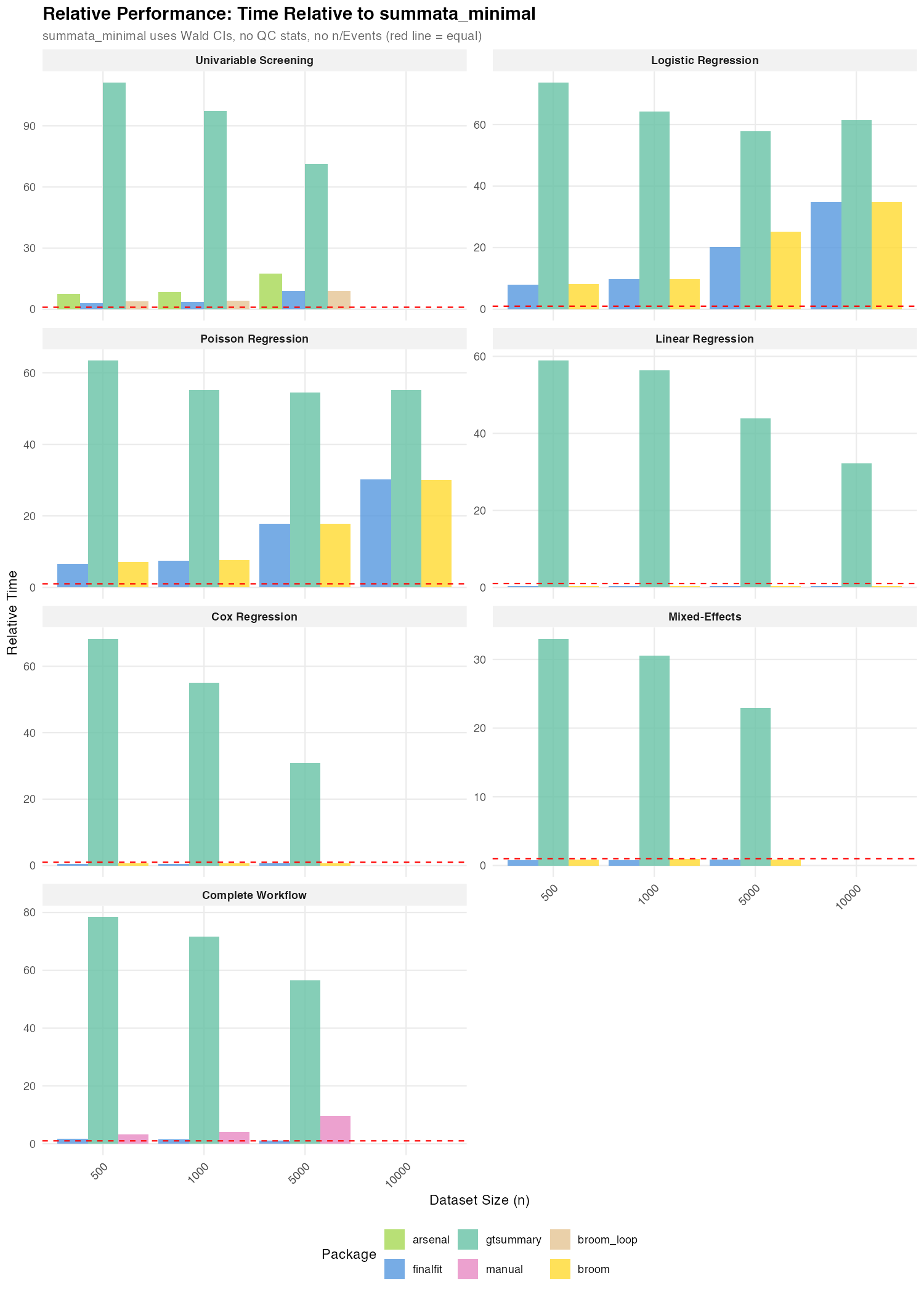
Ratios relative to summata_minimal (Wald CIs):
| Benchmark | gtsummary |
finalfit |
summata (default) |
|---|---|---|---|
| Logistic Regression | 58–74× | 8–35× | 10–34× |
| Poisson Regression | 55–63× | 7–30× | 8–29× |
| Linear Regression | 32–59× | 0.3× | 1.3–1.7× |
| Cox Regression | 31–68× | 0.4–0.6× | 1.5–2.0× |
| Mixed-Effects | 23–33× | 0.8–0.9× | 1.5–1.7× |
| Univariable Screening | 71–111× | 3.1–9.0× | 2.6–3.2× |
| Complete Workflow | 57–78× | 1.1–1.7× | 3.7–7.5× |
For GLM models (logistic and Poisson), summata_minimal
outperforms all alternatives by a wide margin: 8–35× faster than
finalfit, 7–30× faster than broom. This is
because summata_minimal is the only configuration that uses
Wald CIs — finalfit, broom, and the default
summata all use profile likelihood CIs, which accounts for
their comparable timings.
For linear, Cox, and mixed-effects models, where all packages use the
same CI method (exact t-distribution for lm, Wald for Cox and
mixed-effects), the timing gap between summata and
summata_minimal is narrow (1.3–2.0×) and reflects
formatting overhead only.
Scaling Characteristics
The relationship between dataset size and execution time provides
insight into algorithmic complexity. Near-linear scaling (execution time
proportional to n) indicates efficient implementation, while
superlinear scaling may suggest operations with O(n²)
complexity, such as repeated rbind() calls or element-wise
data frame construction.
Observed scaling factors for summata (ratio of time at
n = 10,000 to time at n = 1,000):
| Operation | Scaling Factor | Expected for O(n) |
|---|---|---|
| Descriptive tables | 1.7× | 10× |
| Logistic regression | 6.5× | 10× |
| Univariable screening | 1.8× | 10× |
The sublinear scaling reflects that fixed overhead (package loading, object construction, profile likelihood profiling) constitutes a significant fraction of total time at smaller dataset sizes. Logistic regression shows nearer-to-linear scaling because profile likelihood profiling cost scales with the number of IRLS iterations, which grows with n.
Implementation Notes
The performance characteristics documented here reflect specific implementation choices:
summata: Built on data.table for data
manipulation, with coefficient extraction optimized for common model
classes. Default configuration uses profile likelihood CIs for
GLM/negbin models (matching finalfit and
broom). The conf_method = "wald" option skips
profiling entirely, producing a configuration faster than any
alternative tested.
gtsummary: Prioritizes output flexibility through
the gt table framework. The additional abstraction layers
enable extensive customization but increase computational overhead.
finalfit: Balances functionality and performance
with a tidyverse-compatible interface. Uses profile likelihood CIs by
default for GLM models (confint_type = "profile"). The
finalfit() function is particularly optimized for the
combined workflow.
arsenal: Uses formula-based syntax familiar to SAS users. Performance varies by operation type.
broom: Provides minimal coefficient extraction with
limited formatting. Uses profile likelihood CIs for GLM models via
stats::confint() dispatch. Suitable as a building block for
custom pipelines.
Effect of Output Options
By default, summata regression functions compute profile
likelihood confidence intervals (for GLM and negative binomial models),
sample sizes, event counts, QC statistics, and reference rows for
categorical variables. These features produce more complete and accurate
output for publication but add computational overhead. For
performance-sensitive applications, these options can be disabled.
The summata_minimal configuration shown in the
benchmarks represents:
fit(data, outcome, predictors,
    conf_method = "wald",
    show_n = FALSE,
    show_events = FALSE,
    reference_rows = FALSE,
    keep_qc_stats = FALSE)
The conf_method parameter can also be set globally for
an entire session:
options(summata.conf_method = "wald")The impact of each option varies by model type:
| Option | GLM/negbin models | Linear/Cox/mixed models |
|---|---|---|
conf_method = "wald" |
Large effect (eliminates profile likelihood profiling) | Minimal effect (Wald already used for Cox/mixed; exact t is fast for lm) |
keep_qc_stats = FALSE |
Moderate effect (skips C-statistic, Hosmer-Lemeshow) | Small effect |
show_n/show_events = FALSE |
Small effect | Small effect |
reference_rows = FALSE |
Small effect | Small effect |
For logistic and Poisson models at n = 1,000, the minimal
configuration is approximately 10× faster than the default (22 ms
vs. 234 ms for logistic), with the majority of the difference
attributable to conf_method. For linear and Cox models, the
difference is roughly 1.5–2×, reflecting formatting overhead only.
The choice between configurations depends on the use case:
- Publication tables: Default settings provide profile likelihood CIs and complete output ready for manuscripts
-
Simulation studies:
conf_method = "wald"reduces per-iteration overhead substantially for GLM models -
Exploratory analysis: Either setting is
appropriate;
conf_method = "wald"is recommended when iterating through many model specifications
Practical Considerations
The timing differences documented here range from negligible (tens of milliseconds) to substantial (several seconds). The practical significance depends on context:
- Interactive analysis: Differences under 500 ms are generally imperceptible
- Batch processing: Cumulative differences matter when processing many datasets
- Simulation studies: Per-iteration overhead compounds across thousands of replicates
- Teaching and demonstration: Faster feedback loops improve the interactive experience
Package selection should primarily reflect functional requirements, syntax preferences, and ecosystem compatibility. Performance considerations become relevant only when computational constraints are binding.
Reproducibility
The benchmark script is available in the package repository at
inst/benchmarks/benchmarks.R. Execution produces:
- Individual PNG figures for each benchmark category
- Summary figures (
benchmark_speedup.png,benchmark_speedup_minimal.png) - CSV files with detailed timing data
Results will vary across systems due to differences in hardware, R version, and package versions.
Session Information
This benchmark was run under the following conditions:
R version 4.5.2 (2025-10-31)
Platform: x86_64-unknown-linux-gnu

Matrix products: default
BLAS/LAPACK: /usr/lib/libopenblasp-r0.3.30.so;  LAPACK version 3.12.0

Void Linux x86_64
Linux 6.12.63_1
Intel(R) Core(TM) i5-4670K (4) @ 3.80 GHz
NVIDIA GeForce GTX 970 [Discrete]