Create Publication-Ready Survival Summary Tables

Generates comprehensive survival summary tables with survival probabilities at specified time points, median survival times, and optional group comparisons with statistical testing. Designed for creating survival summaries commonly used in clinical and epidemiological research publications.

Usage

survtable(
  data,
  outcome,
  by = NULL,
  times = NULL,
  probs = 0.5,
  stats = c("survival", "ci"),
  type = "survival",
  conf_level = 0.95,
  conf_type = "log",
  digits = 0,
  time_digits = 1,
  p_digits = 3,
  percent = TRUE,
  test = TRUE,
  test_type = "logrank",
  total = TRUE,
  total_label = "Total",
  time_unit = NULL,
  time_label = NULL,
  median_label = NULL,
  labels = NULL,
  by_label = NULL,
  na_rm = TRUE,
  number_format = NULL,
  ...
)

Arguments

data

Data frame or data.table containing the survival dataset. Automatically converted to a data.table for efficient processing.

outcome

Character string or character vector specifying one or more survival outcomes using Surv() syntax (e.g., "Surv(os_months, os_status)"). When multiple outcomes are provided, results are stacked into a single table with outcome labels as row headers.

by

Character string specifying the column name of the stratifying variable for group comparisons (e.g., treatment arm, risk group). When NULL (default), produces overall survival summaries only.

times

Numeric vector of time points at which to estimate survival probabilities. For example, c(12, 24, 36) for 1-, 2-, and 3-year survival when time is measured in months. Default is NULL.

probs

Numeric vector of survival probabilities for which to estimate corresponding survival times (quantiles). Values must be between 0 and 1. For example, c(0.5) returns median survival time, c(0.25, 0.5, 0.75) returns quartiles. Default is 0.5 (median only).

stats

Character vector specifying which statistics to display:

"survival" - Survival probability at specified times
"ci" - Confidence interval for survival probability
"n_risk" - Number at risk at each time point
"n_event" - Cumulative number of events by each time point

Default is c("survival", "ci").

type

Character string specifying the type of probability to report:

"survival" - Survival probability S(t) [default]
"risk" - Cumulative incidence/risk 1 - S(t)
"cumhaz" - Cumulative hazard -log(S(t))

conf_level

Numeric confidence level for confidence intervals. Must be between 0 and 1. Default is 0.95 (95% confidence intervals).

conf_type

Character string specifying the confidence interval type for survival estimates:

"log" - Log transformation (default, recommended)
"log-log" - Log-log transformation
"plain" - Linear/identity (can produce CIs outside [0, 1])
"logit" - Logit transformation
"arcsin" - Arcsin square root transformation

digits

Integer specifying the number of decimal places for survival probabilities (as percentages). Default is 0 (whole percentages).

time_digits

Integer specifying the number of decimal places for survival time estimates (median, quantiles). Default is 1.

p_digits

Integer specifying the number of decimal places for p-values. Values smaller than 10^(-p_digits) are displayed as "< 0.001" (for p_digits = 3), "< 0.0001" (for p_digits = 4), etc. Default is 3.

percent

Logical. If TRUE (default), displays survival probabilities as percentages (e.g., "85%"). If FALSE, displays as proportions (e.g., "0.85").

test

Logical. If TRUE (default), performs a survival curve comparison test and adds a p-value column. Requires by to be specified.

test_type

Character string specifying the statistical test for comparing survival curves:

"logrank" - Log-rank test (default)
"wilcoxon" - Wilcoxon (Breslow) test
"tarone" - Tarone-Ware test
"petopeto" - Peto-Peto test

total

Logical or character string controlling the total/overall column:

TRUE or "first" - Include total column first [default]
"last" - Include total column last (before p-value)
FALSE - Exclude total column

total_label

Character string for the total/overall row label. Default is "Total".

time_unit

Character string specifying the time unit for display in column headers and labels (e.g., "months", "days", "years"). When specified, time column headers become "{time} {time_unit}" (e.g., "12 months"). Default is NULL (no unit shown).

time_label

Character string template for time column headers when times is specified. Use "\{time\}" as placeholder for the time value and "\{unit\}" for the time unit. Default is "\{time\} \{unit\}" when time_unit is specified, otherwise just "\{time\}".

median_label

Character string for the median survival row label. Default is NULL, which auto-constructs from conf_level (e.g., "Median (95% CI)" for conf_level = 0.95).

labels

Named character vector or list providing custom display labels. For stratified analyses, names should match levels of the by variable. For multiple outcomes, names should match the Surv() expressions. Default is NULL.

by_label

Character string providing a custom label for the stratifying variable (used in output attributes and headers). Default is NULL (uses variable name).

na_rm

Logical. If TRUE (default), observations with missing values in time, status, or the stratifying variable are excluded.

number_format

Character string or two-element character vector controlling thousand and decimal separators in formatted output. Named presets:

"us" - Comma thousands, period decimal: 1,234.56 [default]
"eu" - Period thousands, comma decimal: 1.234,56
"space" - Thin-space thousands, period decimal: 1 234.56 (SI/ISO 31-0)
"none" - No thousands separator: 1234.56

Or provide a custom two-element vector c(big.mark, decimal.mark), e.g., c("'", ".") for Swiss-style: 1'234.56.

When NULL (default), uses getOption("summata.number_format", "us"). Set the global option once per session to avoid passing this argument repeatedly:


    options(summata.number_format = "eu")

...

Additional arguments passed to survfit.

Value

A data.table with S3 class "survtable" containing formatted survival statistics. The table structure depends on parameters:

When times is specified (survival at time points):

Variable/Group: Row identifier – stratifying variable levels
Time columns: Survival statistics at each requested time point
p-value: Test p-value (if test = TRUE and by specified)

When only probs is specified (survival quantiles):

Variable/Group: Row identifier – stratifying variable levels
Quantile columns: Time to reach each survival probability
p-value: Test p-value (if test = TRUE and by specified)

All numeric output (probabilities, times, counts, p-values) respects the number_format setting for locale-appropriate formatting.

The returned object includes the following attributes:

raw_data: Data.table with unformatted numeric values
survfit_objects: List of survfit objects for each stratum
by_variable: The stratifying variable name
times: The time points requested
probs: The probability quantiles requested
test_result: Full test result object (if test performed)

Details

Survival Probability Estimation:

Survival probabilities are estimated using the Kaplan-Meier method via survfit. At each specified time point, the function reports the estimated probability of surviving beyond that time.

Confidence Intervals:

The default "log" transformation for confidence intervals is recommended as it ensures intervals remain within [0, 1] and has good statistical properties. The "log-log" transformation is also commonly used and may perform better in the tails.

Statistical Testing:

The log-rank test (default) tests the null hypothesis that survival curves are identical across groups. Alternative tests weight different parts of the survival curve:

Log-rank: Equal weights (best for proportional hazards)
Wilcoxon: Weights by number at risk (sensitive to early differences)
Tarone-Ware: Weights by square root of number at risk
Peto-Peto: Modified Wilcoxon weights

Formatting:

All numeric output respects the number_format parameter. Separators within confidence intervals adapt automatically to avoid ambiguity:

Survival probabilities: "85% (80%-89%)" (US) or "85% (80%-89%)" (EU, en-dash separator)
Median survival: "24.5 (21.2-28.9)" (US) or "24,5 (21,2-28,9)" (EU)
Counts \(\ge\) 1000: "1,234" (US) or "1.234" (EU)
p-values: "< 0.001" (US) or "< 0,001" (EU)

Examples

# Load example data
data(clintrial)

# Example 1: Survival at specific time points by treatment
survtable(
    data = clintrial,
    outcome = "Surv(os_months, os_status)",
    by = "treatment",
    times = c(12, 24, 36),
    time_unit = "months"
)
#> 
#> Survival Summary Table
#> Outcome: Surv(os_months, os_status)
#> Stratified by: treatment
#> Time points: 12, 24, 36 months
#> Quantiles: 50%
#> Statistic: Survival probability
#> Test: Log-rank (p = < 0.001)
#> 
#>    Variable    12 months    24 months    36 months  Median (95% CI) p-value
#>      <char>       <char>       <char>       <char>           <char>  <char>
#> 1:    Total 59% (56-62%) 46% (43-49%) 36% (33-40%) 19.4 (16.2-23.4) < 0.001
#> 2:  Control 55% (49-63%) 37% (31-44%) 26% (20-33%) 14.7 (10.5-19.2)        
#> 3:   Drug A 68% (63-74%) 56% (51-62%) 48% (42-54%) 33.6 (24.5-42.2)        
#> 4:   Drug B 54% (49-59%) 43% (38-48%) 33% (28-38%) 14.7 (11.0-21.8)        

# \donttest{

# Example 2: Median survival only
survtable(
    data = clintrial,
    outcome = "Surv(os_months, os_status)",
    by = "treatment",
    times = NULL,
    probs = 0.5
)
#> 
#> Survival Summary Table
#> Outcome: Surv(os_months, os_status)
#> Stratified by: treatment
#> Quantiles: 50%
#> Statistic: Survival probability
#> Test: Log-rank (p = < 0.001)
#> 
#>    Variable  Median (95% CI) p-value
#>      <char>           <char>  <char>
#> 1:    Total 19.4 (16.2-23.4) < 0.001
#> 2:  Control 14.7 (10.5-19.2)        
#> 3:   Drug A 33.6 (24.5-42.2)        
#> 4:   Drug B 14.7 (11.0-21.8)        

# Example 3: Multiple quantiles (quartiles)
survtable(
    data = clintrial,
    outcome = "Surv(os_months, os_status)",
    by = "stage",
    times = NULL,
    probs = c(0.25, 0.5, 0.75)
)
#> 
#> Survival Summary Table
#> Outcome: Surv(os_months, os_status)
#> Stratified by: stage
#> Quantiles: 25%, 50%, 75%
#> Statistic: Survival probability
#> Test: Log-rank (p = < 0.001)
#> 
#>    Variable 75% Survival Time (95% CI)  Median (95% CI) 25% Survival Time (95% CI) p-value
#>      <char>                     <char>           <char>                     <char>  <char>
#> 1:    Total              5.1 (4.3-6.1) 19.5 (16.1-23.5)                         NR < 0.001
#> 2:        I             9.0 (7.4-12.5) 33.7 (22.4-45.2)                         NR        
#> 3:       II             7.7 (6.1-12.3) 32.2 (24.8-42.0)                         NR        
#> 4:      III              3.9 (3.0-5.2) 13.7 (10.4-22.3)             44.7 (35.8-NR)        
#> 5:       IV              2.0 (1.4-2.8)    5.9 (4.3-8.2)           15.6 (10.8-26.7)        

# Example 4: Both time points and median
survtable(
    data = clintrial,
    outcome = "Surv(os_months, os_status)",
    by = "treatment",
    times = c(12, 24),
    probs = 0.5,
    time_unit = "months"
)
#> 
#> Survival Summary Table
#> Outcome: Surv(os_months, os_status)
#> Stratified by: treatment
#> Time points: 12, 24 months
#> Quantiles: 50%
#> Statistic: Survival probability
#> Test: Log-rank (p = < 0.001)
#> 
#>    Variable    12 months    24 months  Median (95% CI) p-value
#>      <char>       <char>       <char>           <char>  <char>
#> 1:    Total 59% (56-62%) 46% (43-49%) 19.4 (16.2-23.4) < 0.001
#> 2:  Control 55% (49-63%) 37% (31-44%) 14.7 (10.5-19.2)        
#> 3:   Drug A 68% (63-74%) 56% (51-62%) 33.6 (24.5-42.2)        
#> 4:   Drug B 54% (49-59%) 43% (38-48%) 14.7 (11.0-21.8)        

# Example 5: Cumulative incidence (1 - survival)
survtable(
    data = clintrial,
    outcome = "Surv(os_months, os_status)",
    by = "treatment",
    times = c(12, 24),
    type = "risk"
)
#> 
#> Survival Summary Table
#> Outcome: Surv(os_months, os_status)
#> Stratified by: treatment
#> Time points: 12, 24
#> Quantiles: 50%
#> Statistic: Cumulative incidence
#> Test: Log-rank (p = < 0.001)
#> 
#>    Variable           12           24  Median (95% CI) p-value
#>      <char>       <char>       <char>           <char>  <char>
#> 1:    Total 41% (38-44%) 54% (51-57%) 19.4 (16.2-23.4) < 0.001
#> 2:  Control 45% (37-51%) 63% (56-69%) 14.7 (10.5-19.2)        
#> 3:   Drug A 32% (26-37%) 44% (38-49%) 33.6 (24.5-42.2)        
#> 4:   Drug B 46% (41-51%) 57% (52-62%) 14.7 (11.0-21.8)        

# Example 6: Include number at risk
survtable(
    data = clintrial,
    outcome = "Surv(os_months, os_status)",
    by = "treatment",
    times = c(12, 24),
    stats = c("survival", "ci", "n_risk")
)
#> 
#> Survival Summary Table
#> Outcome: Surv(os_months, os_status)
#> Stratified by: treatment
#> Time points: 12, 24
#> Quantiles: 50%
#> Statistic: Survival probability
#> Test: Log-rank (p = < 0.001)
#> 
#>    Variable                     12                     24  Median (95% CI) p-value
#>      <char>                 <char>                 <char>           <char>  <char>
#> 1:    Total 59% (56-62%) [n = 488] 46% (43-49%) [n = 369] 19.4 (16.2-23.4) < 0.001
#> 2:  Control 55% (49-63%) [n = 106]  37% (31-44%) [n = 70] 14.7 (10.5-19.2)        
#> 3:   Drug A 68% (63-74%) [n = 192] 56% (51-62%) [n = 154] 33.6 (24.5-42.2)        
#> 4:   Drug B 54% (49-59%) [n = 190] 43% (38-48%) [n = 145] 14.7 (11.0-21.8)        

# Example 7: Overall survival without stratification
survtable(
    data = clintrial,
    outcome = "Surv(os_months, os_status)",
    times = c(12, 24, 36, 48)
)
#> 
#> Survival Summary Table
#> Outcome: Surv(os_months, os_status)
#> Time points: 12, 24, 36, 48
#> Quantiles: 50%
#> Statistic: Survival probability
#> 
#>    Variable           12           24           36           48  Median (95% CI)
#>      <char>       <char>       <char>       <char>       <char>           <char>
#> 1:    Total 59% (56-62%) 46% (43-49%) 36% (33-40%) 30% (27-33%) 19.4 (16.2-23.4)

# Example 8: Without total row
survtable(
    data = clintrial,
    outcome = "Surv(os_months, os_status)",
    by = "treatment",
    times = c(12, 24),
    total = FALSE
)
#> 
#> Survival Summary Table
#> Outcome: Surv(os_months, os_status)
#> Stratified by: treatment
#> Time points: 12, 24
#> Quantiles: 50%
#> Statistic: Survival probability
#> Test: Log-rank (p = < 0.001)
#> 
#>    Variable           12           24  Median (95% CI) p-value
#>      <char>       <char>       <char>           <char>  <char>
#> 1:  Control 55% (49-63%) 37% (31-44%) 14.7 (10.5-19.2) < 0.001
#> 2:   Drug A 68% (63-74%) 56% (51-62%) 33.6 (24.5-42.2)        
#> 3:   Drug B 54% (49-59%) 43% (38-48%) 14.7 (11.0-21.8)        

# Example 9: Custom labels
survtable(
    data = clintrial,
    outcome = "Surv(os_months, os_status)",
    by = "treatment",
    times = c(12, 24),
    labels = c("Drug A" = "Treatment A", "Drug B" = "Treatment B"),
    time_unit = "months"
)
#> 
#> Survival Summary Table
#> Outcome: Surv(os_months, os_status)
#> Stratified by: treatment
#> Time points: 12, 24 months
#> Quantiles: 50%
#> Statistic: Survival probability
#> Test: Log-rank (p = < 0.001)
#> 
#>       Variable    12 months    24 months  Median (95% CI) p-value
#>         <char>       <char>       <char>           <char>  <char>
#> 1:       Total 59% (56-62%) 46% (43-49%) 19.4 (16.2-23.4) < 0.001
#> 2:     Control 55% (49-63%) 37% (31-44%) 14.7 (10.5-19.2)        
#> 3: Treatment A 68% (63-74%) 56% (51-62%) 33.6 (24.5-42.2)        
#> 4: Treatment B 54% (49-59%) 43% (38-48%) 14.7 (11.0-21.8)        

# Example 10: Different confidence interval type
survtable(
    data = clintrial,
    outcome = "Surv(os_months, os_status)",
    by = "treatment",
    times = c(12, 24),
    conf_type = "log-log"
)
#> 
#> Survival Summary Table
#> Outcome: Surv(os_months, os_status)
#> Stratified by: treatment
#> Time points: 12, 24
#> Quantiles: 50%
#> Statistic: Survival probability
#> Test: Log-rank (p = < 0.001)
#> 
#>    Variable           12           24  Median (95% CI) p-value
#>      <char>       <char>       <char>           <char>  <char>
#> 1:    Total 59% (56-62%) 46% (42-49%) 19.4 (16.1-22.9) < 0.001
#> 2:  Control 55% (48-62%) 37% (30-44%) 14.7 (10.2-19.0)        
#> 3:   Drug A 68% (63-73%) 56% (50-62%) 33.6 (24.4-40.9)        
#> 4:   Drug B 54% (48-59%) 43% (38-48%) 14.7 (10.9-21.7)        

# Example 11: Wilcoxon test instead of log-rank
survtable(
    data = clintrial,
    outcome = "Surv(os_months, os_status)",
    by = "treatment",
    times = c(12, 24),
    test_type = "wilcoxon"
)
#> 
#> Survival Summary Table
#> Outcome: Surv(os_months, os_status)
#> Stratified by: treatment
#> Time points: 12, 24
#> Quantiles: 50%
#> Statistic: Survival probability
#> Test: Wilcoxon (p = < 0.001)
#> 
#>    Variable           12           24  Median (95% CI) p-value
#>      <char>       <char>       <char>           <char>  <char>
#> 1:    Total 59% (56-62%) 46% (43-49%) 19.4 (16.2-23.4) < 0.001
#> 2:  Control 55% (49-63%) 37% (31-44%) 14.7 (10.5-19.2)        
#> 3:   Drug A 68% (63-74%) 56% (51-62%) 33.6 (24.5-42.2)        
#> 4:   Drug B 54% (49-59%) 43% (38-48%) 14.7 (11.0-21.8)        

# Example 12: Access raw data for custom analysis
result <- survtable(
    data = clintrial,
    outcome = "Surv(os_months, os_status)",
    by = "treatment",
    times = c(12, 24)
)
raw <- attr(result, "raw_data")
print(raw)
#>    Variable 12_estimate  12_lower  12_upper 12_n_risk 12_n_event 24_estimate  24_lower  24_upper 24_n_risk 24_n_event Median (95% CI)_estimate Median (95% CI)_lower Median (95% CI)_upper
#>      <char>       <num>     <num>     <num>     <num>      <num>       <num>     <num>     <num>     <num>      <num>                    <num>                 <num>                 <num>
#> 1:    Total   0.5897650 0.5573977 0.6240118       488        345   0.4589077 0.4262187 0.4941037       369        107                     19.4                  16.2                  23.4
#> 2:  Control   0.5518225 0.4860549 0.6264890       106         87   0.3686484 0.3063818 0.4435696        70         35                     14.7                  10.5                  19.2
#> 3:   Drug A   0.6829195 0.6310704 0.7390285       192         91   0.5604338 0.5054384 0.6214131       154         34                     33.6                  24.5                  42.2
#> 4:   Drug B   0.5361330 0.4869622 0.5902688       190        167   0.4272844 0.3788226 0.4819458       145         38                     14.7                  11.0                  21.8

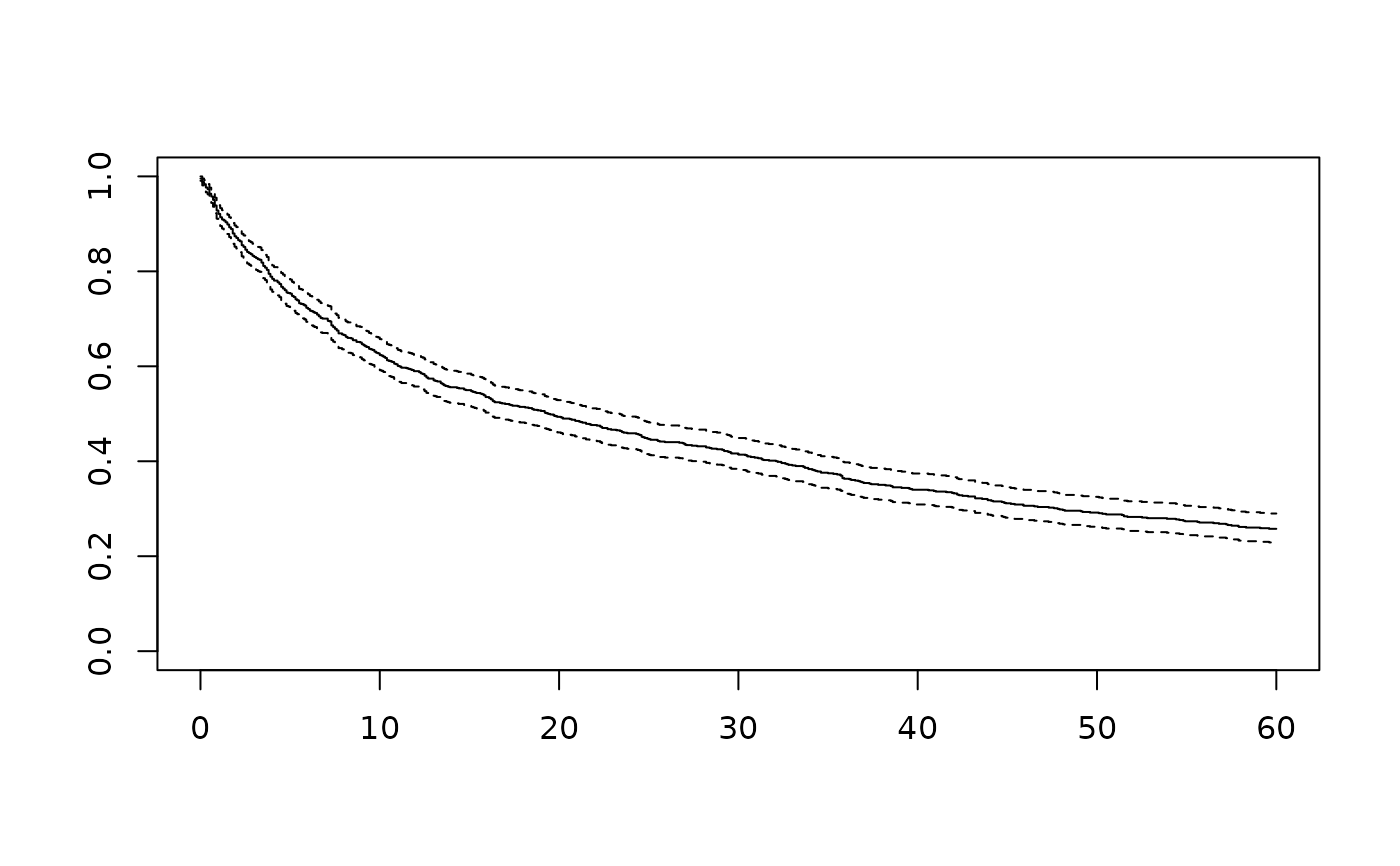
# Example 13: Access survfit objects for plotting
fits <- attr(result, "survfit_objects")
plot(fits$overall)  # Plot overall survival curve


# Example 14: Multiple survival outcomes stacked
survtable(
    data = clintrial,
    outcome = c("Surv(pfs_months, pfs_status)", "Surv(os_months, os_status)"),
    by = "treatment",
    times = c(12, 24),
    probs = 0.5,
    time_unit = "months",
    total = FALSE,
    labels = c(
        "Surv(pfs_months, pfs_status)" = "Progression-Free Survival",
        "Surv(os_months, os_status)" = "Overall Survival"
    )
)
#> 
#> Survival Summary Table
#> Outcomes: 2
#> Stratified by: treatment
#> Time points: 12, 24 months
#> Quantiles: 50%
#> Statistic: Survival probability
#> Test: Log-rank
#> 
#>                     Variable   Group    12 months    24 months  Median (95% CI) p-value
#>                       <char>  <char>       <char>       <char>           <char>  <char>
#> 1: Progression-Free Survival Control 29% (23-36%)  14% (9-20%)    4.7 (3.6-6.9) < 0.001
#> 2:                            Drug A 44% (39-51%) 30% (25-36%)   9.0 (7.5-12.4)        
#> 3:                            Drug B 30% (26-36%) 18% (14-22%)    4.7 (3.7-6.2)        
#> 4:          Overall Survival Control 55% (49-63%) 37% (31-44%) 14.7 (10.5-19.2) < 0.001
#> 5:                            Drug A 68% (63-74%) 56% (51-62%) 33.6 (24.5-42.2)        
#> 6:                            Drug B 54% (49-59%) 43% (38-48%) 14.7 (11.0-21.8)        

# Example 15: European number formatting
survtable(
    data = clintrial,
    outcome = "Surv(os_months, os_status)",
    by = "treatment",
    times = c(12, 24),
    number_format = "eu"
)
#> 
#> Survival Summary Table
#> Outcome: Surv(os_months, os_status)
#> Stratified by: treatment
#> Time points: 12, 24
#> Quantiles: 50%
#> Statistic: Survival probability
#> Test: Log-rank (p = < 0.001)
#> 
#>    Variable           12           24  Median (95% CI) p-value
#>      <char>       <char>       <char>           <char>  <char>
#> 1:    Total 59% (56–62%) 46% (43–49%) 19,4 (16,2–23,4) < 0,001
#> 2:  Control 55% (49–63%) 37% (31–44%) 14,7 (10,5–19,2)        
#> 3:   Drug A 68% (63–74%) 56% (51–62%) 33,6 (24,5–42,2)        
#> 4:   Drug B 54% (49–59%) 43% (38–48%) 14,7 (11,0–21,8)        

# }