Forest Plots

Forest plots provide a graphical representation of effect estimates and their precision. Each row displays a point estimate (typically an odds ratio, hazard ratio, or regression coefficient) with a confidence interval, enabling rapid visual assessment of effect magnitude, direction, and statistical significance. The format is standard in published research and regulatory submissions.

The summata package provides specialized forest plot functions for each model type, plus an automatic detection function:

Function	Model Type	Effect Measure
lmforest()	Linear regression	Coefficient (β)
glmforest()	Logistic/Poisson	Odds ratio / Rate ratio
coxforest()	Cox regression	Hazard ratio
uniforest()	Univariable screening	Model-dependent
multiforest()	Multi-outcome analysis	Model-dependent
autoforest()	Auto-detect	Auto-detect

These functions follow a standard syntax when called:

forest_plot <- autoforest(x, data, ...)

where x is either a model or a summata fitted output (e.g., from uniscreen(), fit(), fullfit(), or multifit()), and data is the name of the dataset used. The data argument is optional and is primarily used to derive n and Events counts for various groups/subgroups.

All forest plot functions produce ggplot2 objects that can be further customized. This vignette demonstrates the various capabilities of these functions using the included sample dataset.

---

Preliminaries

The examples in this vignette use the clintrial dataset included with summata:

library(summata)
library(survival)
library(ggplot2)

data(clintrial)
data(clintrial_labels)

n.b.: To ensure correct font rendering and figure sizing, the forest plots below are displayed using a helper function (queue_plot()) that applies each plot’s recommended dimensions (stored in the "rec_dims" attribute) via the ragg graphics device. In practice, replace queue_plot() with ggplot2::ggsave() using recommended plot dimensions for equivalent results:

p <- glmforest(model, data = mydata)
dims <- attr(p, "rec_dims")
ggplot2::ggsave("forest_plot.png", p,
                width = dims$width, 
                height = dims$height)

This ensures that the figure size is always large enough to accommodate the constituent plot text and graphics, and it is generally the preferred method for saving forest plot outputs in summata.

---

Creating Forest Plots from Model Objects

Forest plots can be created from standard R model objects or from summata function output.

Example 1: Logistic Regression

Fit a model using base R, then create a forest plot:

logistic_model <- glm(
  surgery ~ age + sex + stage + treatment + ecog,
  data = clintrial,
  family = binomial
)

example1 <- glmforest(
  x = logistic_model,
  data = clintrial,
  title = "Logistic Regression: Predictors of Outcome",
  labels = clintrial_labels
)
queue_plot(example1)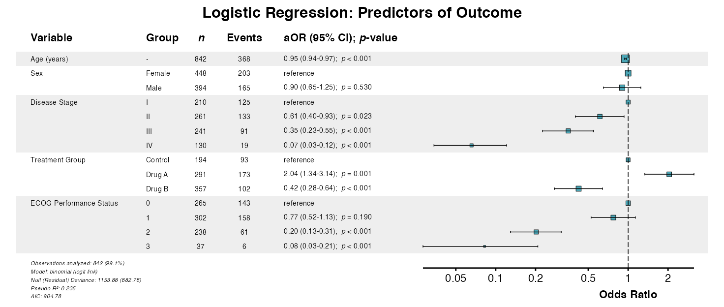

Example 2: Linear Regression

For continuous outcomes, use lmforest():

linear_model <- lm(
  los_days ~ age + sex + stage + surgery + ecog,
  data = clintrial
)

example2 <- lmforest(
  x = linear_model,
  data = clintrial,
  title = "Linear Regression: Length of Stay",
  labels = clintrial_labels
)
queue_plot(example2)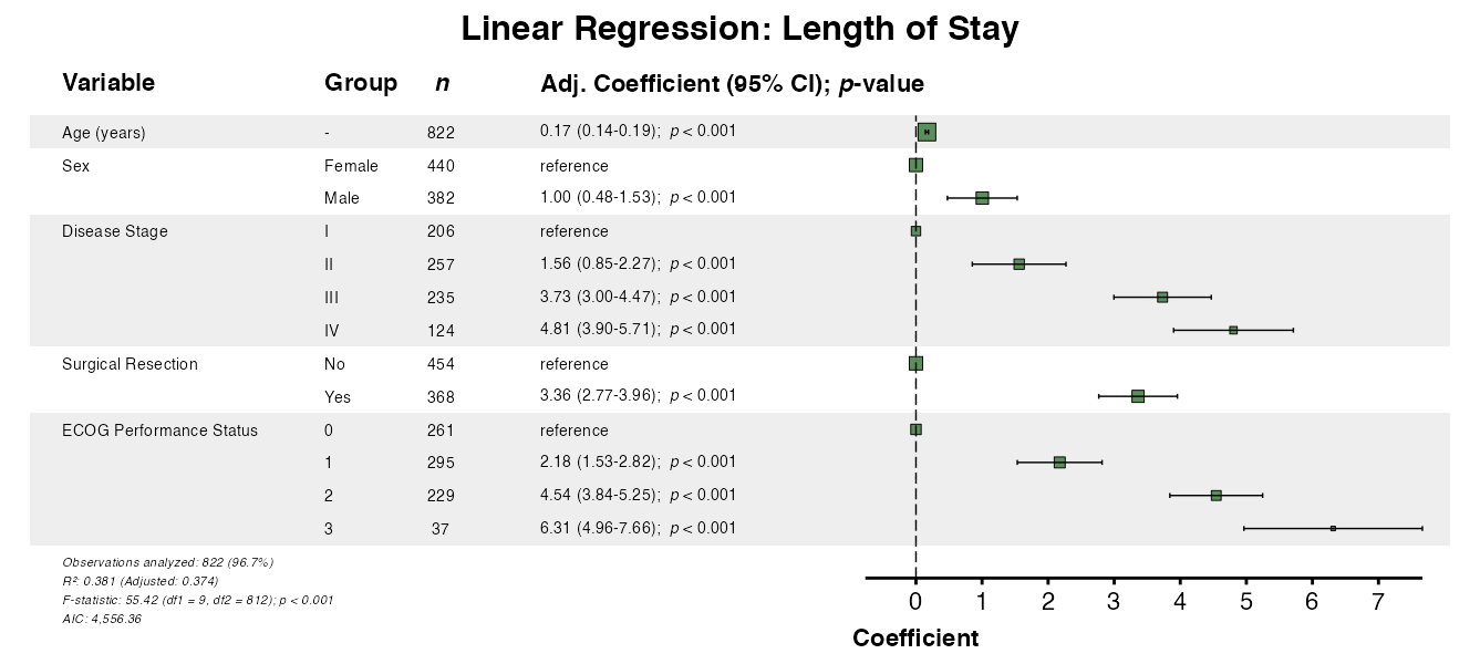

Example 3: Cox Regression

For survival models, use coxforest():

cox_model <- coxph(
  Surv(os_months, os_status) ~ age + sex + stage + treatment + ecog,
  data = clintrial
)

example3 <- coxforest(
  x = cox_model,
  data = clintrial,
  title = "Cox Regression: Survival Analysis",
  labels = clintrial_labels
)
queue_plot(example3)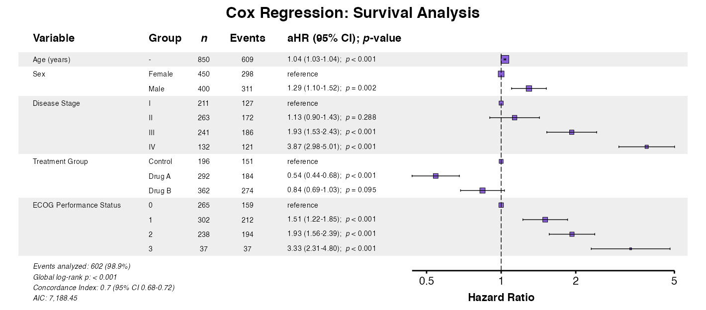

Example 4: Automatic Model Detection

The autoforest() function detects the model type automatically:

example4 <- autoforest(
  x = cox_model,
  data = clintrial,
  labels = clintrial_labels
)
queue_plot(example4)

---

Creating Forest Plots from summata Output

Forest plots integrate seamlessly with fit() and fullfit() output by extracting the attached model object.

Example 5: Direct Extraction from Fit Output

The same approach works for logistic models:

table_logistic <- fit(
  data = clintrial,
  outcome = "surgery",
  predictors = c("age", "sex", "stage", "treatment", "ecog"),
  model_type = "glm",
  labels = clintrial_labels
)

example5 <- glmforest(
  x = attr(table_logistic, "model"),
  title = "Predictors of Surgical Intervention",
  labels = clintrial_labels,
  zebra_stripes = TRUE
)
queue_plot(example5)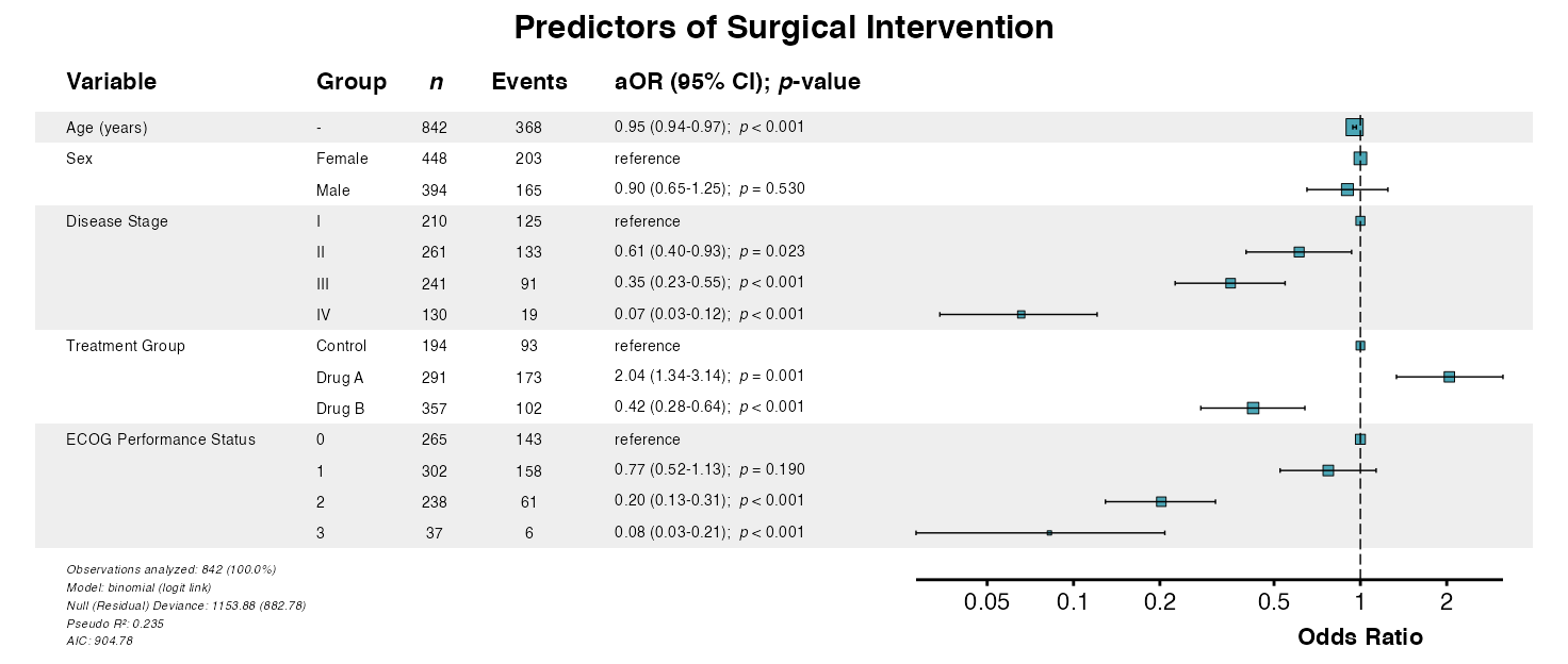

Example 6: Model Attribute from Fit Output

And for Cox models:

table_cox <- fit(
  data = clintrial,
  outcome = "Surv(os_months, os_status)",
  predictors = c("age", "sex", "stage", "treatment", "ecog"),
  model_type = "coxph",
  labels = clintrial_labels
)

example6 <- coxforest(
  x = attr(table_cox, "model"),
  title = "Predictors of Overall Survival",
  labels = clintrial_labels,
  zebra_stripes = TRUE
)
queue_plot(example6)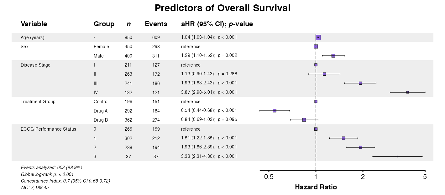

---

Display Options

Example 7: Indenting Factor Levels

The indent_groups parameter creates hierarchical display for a more compact aesthetic:

example7 <- glmforest(
  x = attr(table_logistic, "model"),
  title = "Indented Factor Levels",
  labels = clintrial_labels,
  indent_groups = TRUE
)
queue_plot(example7)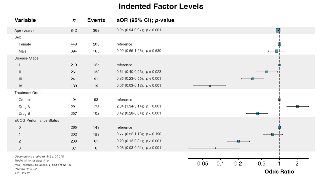

Example 8: Condensing Binary Variables

The condense_table parameter displays binary variables on single rows. Group indenting is applied automatically:

example8 <- glmforest(
  x = attr(table_logistic, "model"),
  title = "Condensed Display",
  labels = clintrial_labels,
  condense_table = TRUE
)
queue_plot(example8)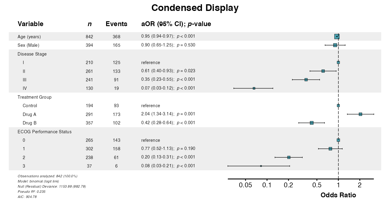

Example 9: Toggle Zebra Striping

Zebra striping is enabled by default. It can be disabled via zebra_stripes = FALSE:

example9 <- glmforest(
  x = attr(table_logistic, "model"),
  title = "Without Zebra Striping",
  labels = clintrial_labels,
  indent_groups = TRUE,
  zebra_stripes = FALSE
)
queue_plot(example9)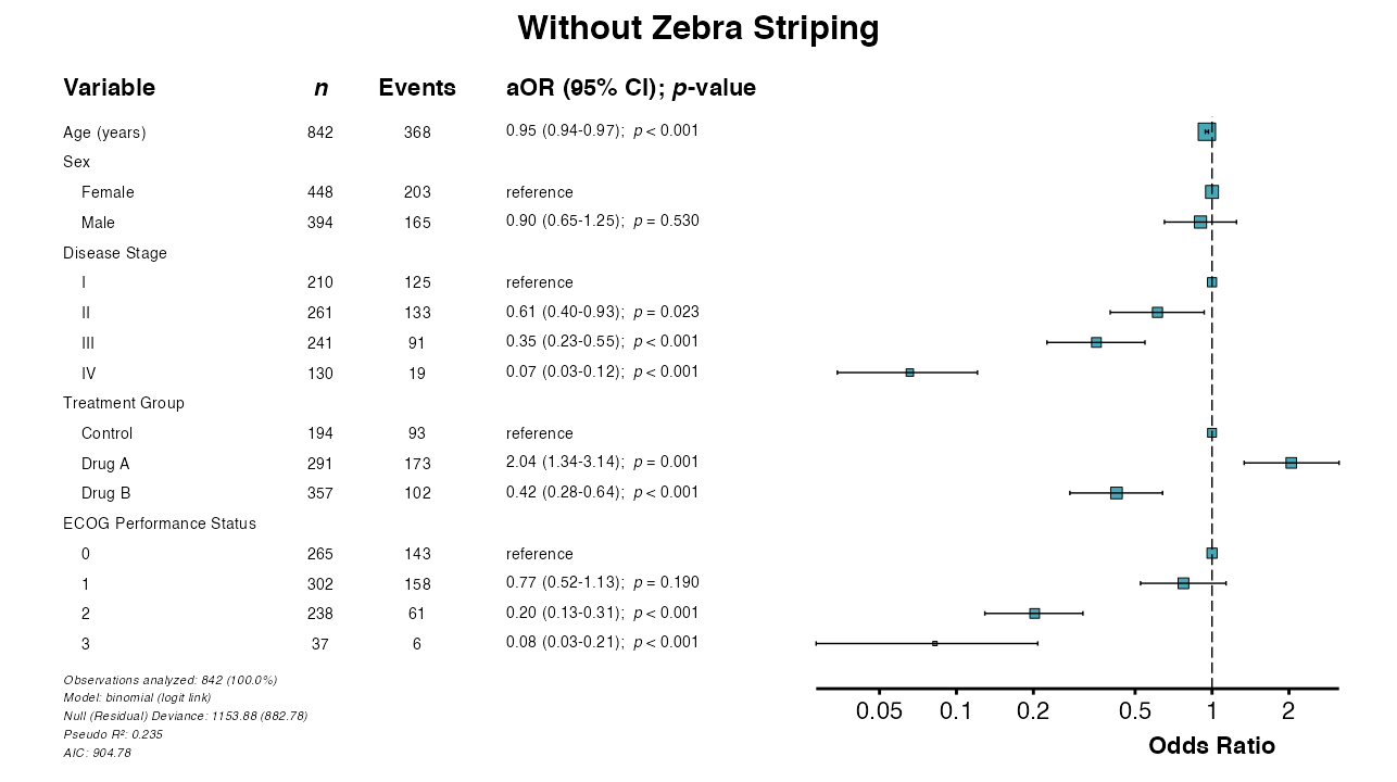

Example 10: Sample Size and Event Columns

Control display of sample size (n) and event counts:

# Show both n and events
example10a <- coxforest(
  x = attr(table_cox, "model"),
  title = "With Sample Size and Events",
  labels = clintrial_labels,
  show_n = TRUE,
  show_events = TRUE,
  indent_groups = TRUE,
  zebra_stripes = TRUE
)
queue_plot(example10a)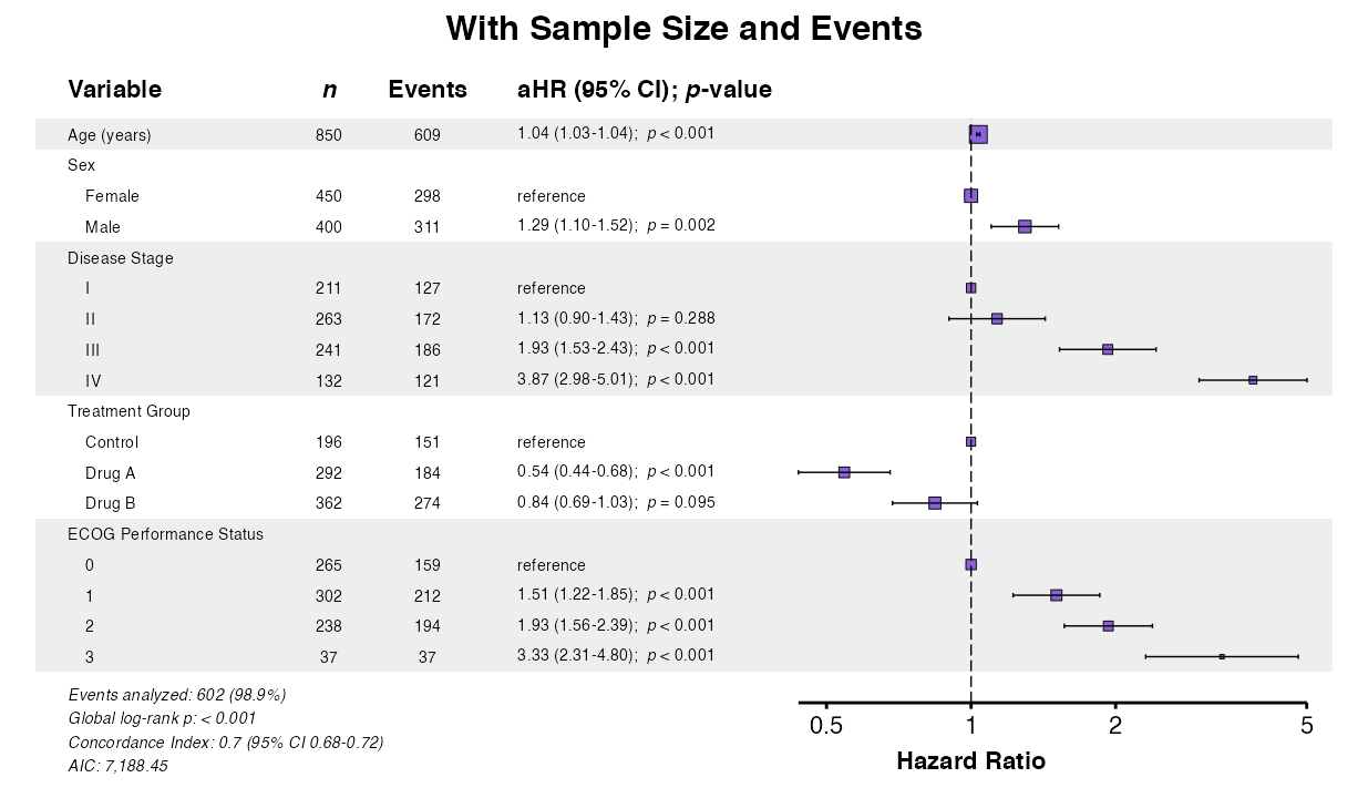

# Minimal display
example10b <- coxforest(
  x = attr(table_cox, "model"),
  title = "Minimal Display",
  labels = clintrial_labels,
  show_n = FALSE,
  show_events = FALSE,
  indent_groups = TRUE
)
queue_plot(example10b)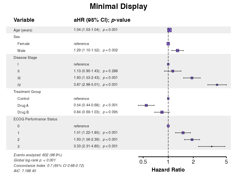

---

Formatting Options

Example 11: Adjusting Numeric Precision

The digits parameter controls decimal places for effect estimates and confidence intervals:

example11 <- glmforest(
  x = attr(table_logistic, "model"),
  title = "Custom Precision (3 decimal places)",
  labels = clintrial_labels,
  digits = 3,
  indent_groups = TRUE
)
queue_plot(example11)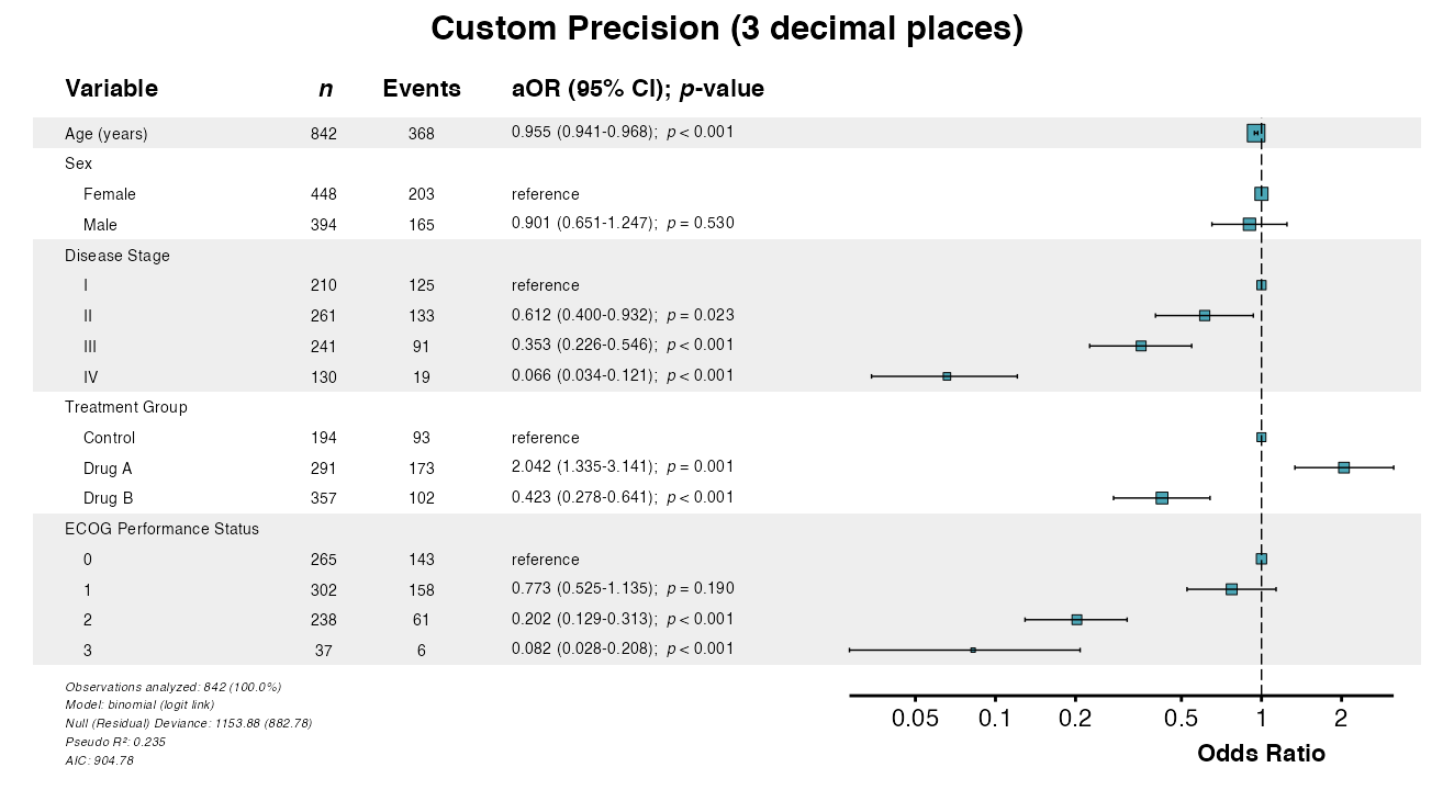

Example 12: Custom Reference Label

Customize the label shown for reference categories:

example12 <- glmforest(
  x = attr(table_logistic, "model"),
  title = "Custom Reference Label",
  labels = clintrial_labels,
  ref_label = "ref",
  indent_groups = TRUE
)
queue_plot(example12)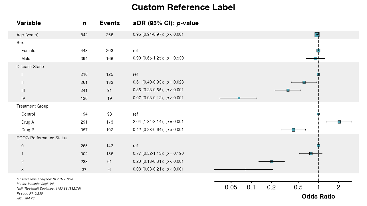

Example 13: Custom Effect Measure Label

Change the column header for the effect measure:

example13 <- coxforest(
  x = attr(table_cox, "model"),
  title = "Custom Effect Label",
  labels = clintrial_labels,
  effect_label = "Effect (95% CI)",
  indent_groups = TRUE
)
queue_plot(example13)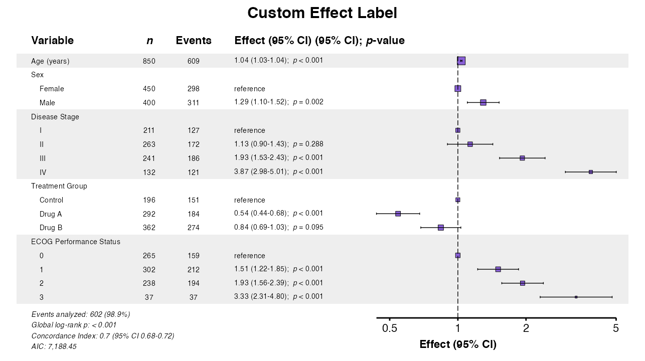

Example 14: Custom Colors

The color parameter changes the point and line color:

example14 <- glmforest(
  x = attr(table_logistic, "model"),
  title = "Custom Color",
  labels = clintrial_labels,
  color = "#E41A1C",
  indent_groups = TRUE
)
queue_plot(example14)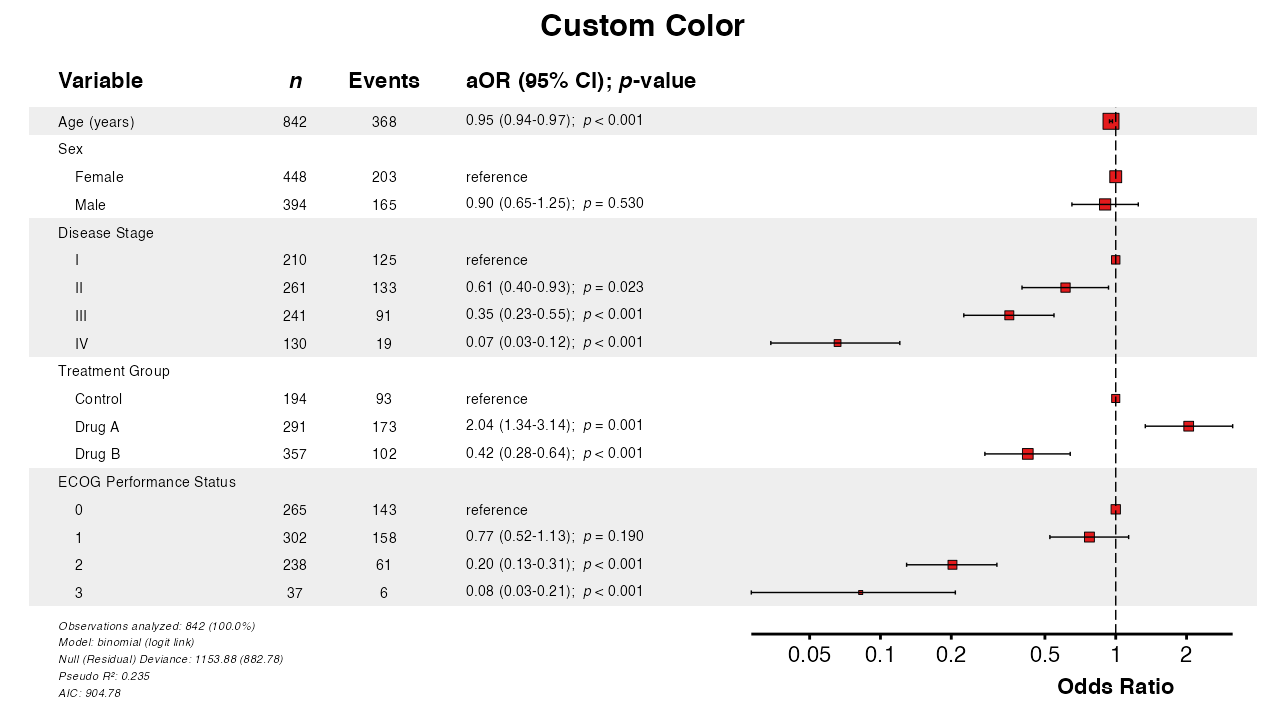

Example 15: Change Font Sizes

Adjust text size with the font_size multiplier:

example15 <- glmforest(
  x = attr(table_logistic, "model"),
  title = "Larger Font (1.5×)",
  labels = clintrial_labels,
  font_size = 1.5,
  indent_groups = TRUE
)
queue_plot(example15)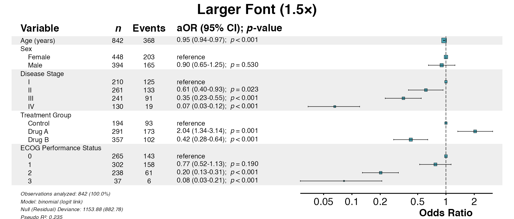

Example 16: Table Width

The table_width parameter adjusts the proportion of space allocated to the table vs. the forest plot:

# Wide table (for long variable names)
example16a <- glmforest(
  x = attr(table_logistic, "model"),
  title = "Wide Table (75%)",
  labels = clintrial_labels,
  table_width = 0.75
)
queue_plot(example16a)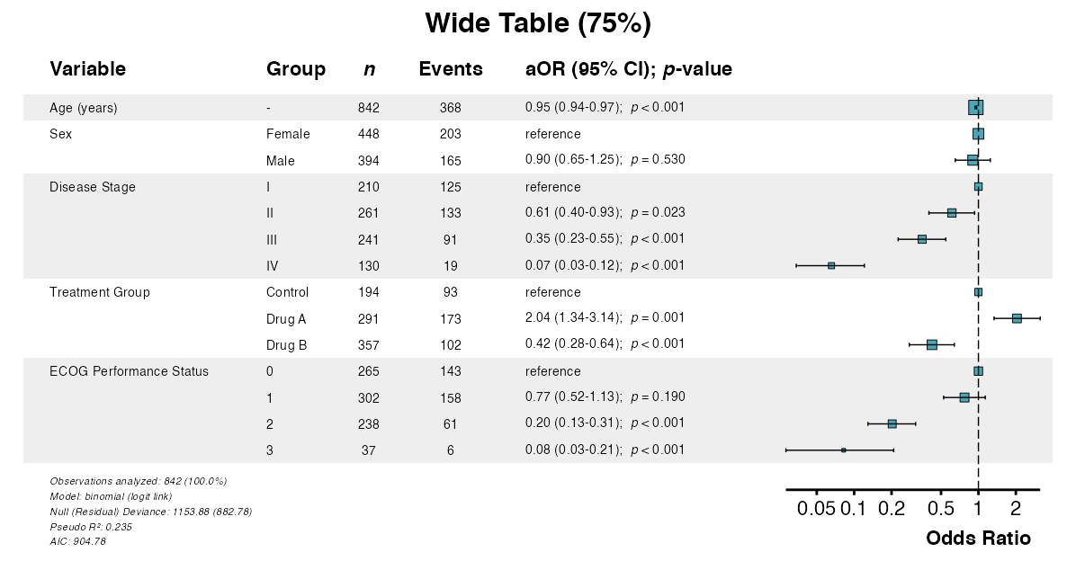

# Narrow table (emphasizes forest plot)
example16b <- glmforest(
  x = attr(table_logistic, "model"),
  title = "Narrow Table (50%)",
  labels = clintrial_labels,
  table_width = 0.50
)
queue_plot(example16b)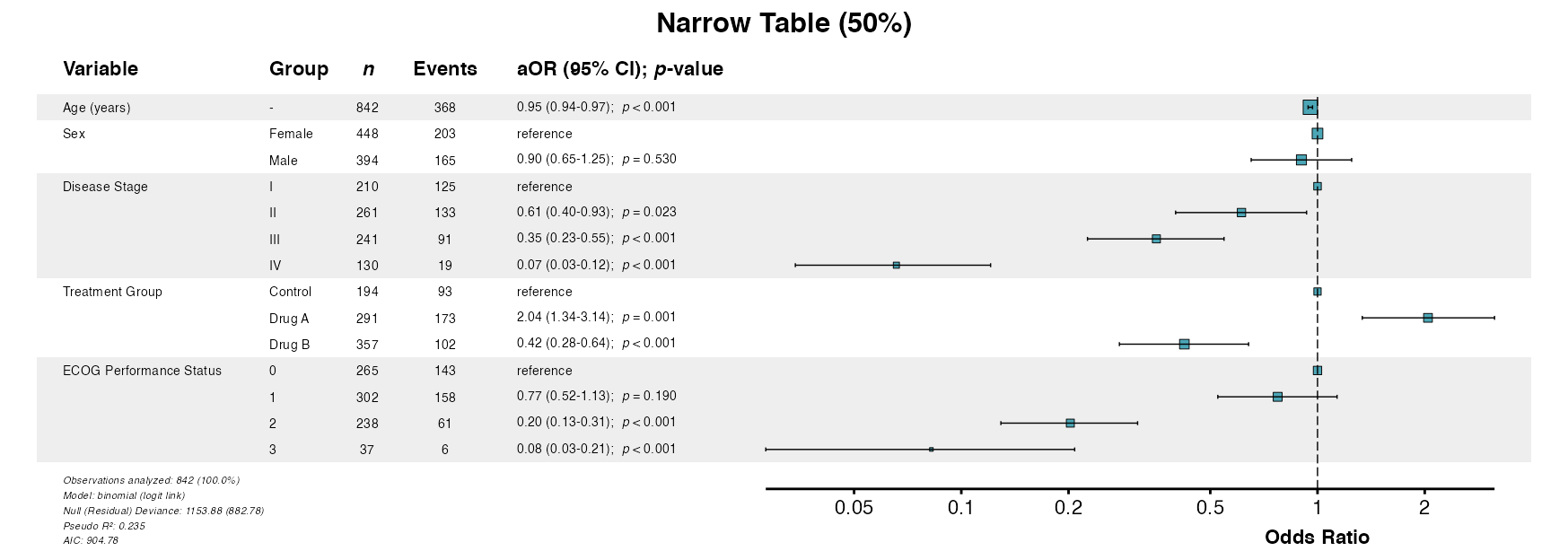

---

Saving Forest Plots

Forest plots include a rec_dims attribute for optimal sizing when saving to files.

Example 17: Recommended Dimensions

Use the recommended dimensions for optimal output:

p <- glmforest(
  x = attr(table_logistic, "model"),
  title = "Publication-Ready Plot",
  labels = clintrial_labels,
  indent_groups = TRUE,
  zebra_stripes = TRUE
)

# Get recommended dimensions
dims <- attr(p, "rec_dims")
cat("Width:", dims$width, "inches\n")
cat("Height:", dims$height, "inches\n")

# Save with recommended dimensions
ggsave(
  filename = file.path(tempdir(), "forest_plot.pdf"),
  plot = p,
  width = dims$width,
  height = dims$height,
  units = "in"
)

Example 18: Multiple Formats

Export to different formats as needed:

p <- glmforest(
  x = attr(table_logistic, "model"),
  title = "Forest Plot",
  labels = clintrial_labels
)

dims <- attr(p, "rec_dims")

# PDF (vector, best for publications)
ggsave("forest.pdf", p, width = dims$width, height = dims$height)

# PNG (raster, good for presentations)
ggsave("forest.png", p, width = dims$width, height = dims$height, dpi = 300)

# TIFF (high-quality raster, often required by journals)
ggsave("forest.tiff", p, width = dims$width, height = dims$height, dpi = 300)

# SVG (vector, good for web)
ggsave("forest.svg", p, width = dims$width, height = dims$height)

---

Advanced Customization

Forest plots support extensive customization for publication requirements.

Example 19: Combined Options

Combine multiple options for publication-ready output:

example19 <- coxforest(
  x = attr(table_cox, "model"),
  title = "Comprehensive Survival Analysis",
  labels = clintrial_labels,
  effect_label = "Hazard Ratio",
  digits = 2,
  show_n = TRUE,
  show_events = TRUE,
  indent_groups = TRUE,
  condense_table = FALSE,
  zebra_stripes = TRUE,
  ref_label = "reference",
  font_size = 1.0,
  table_width = 0.62,
  color = "#8A61D8"
)
queue_plot(example19)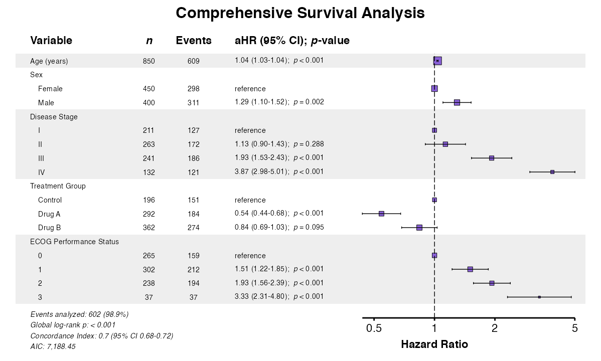

Example 20: Extensions with ggplot2

Forest plots are ggplot2 objects and can be modified further:

example20 <- glmforest(
  x = attr(table_logistic, "model"),
  title = "Extended with ggplot2",
  labels = clintrial_labels,
  indent_groups = TRUE
)

example20_modified <- example20 +
  theme(
    plot.title = element_text(face = "italic", color = "#A72727"),
    plot.background = element_rect(fill = "white", color = NA)
  )
queue_plot(example20_modified)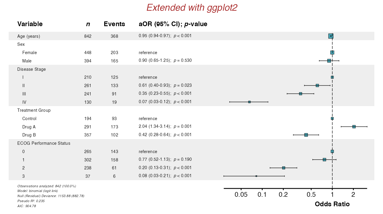

---

Additional GLM Families

The glmforest() function supports all GLM families. These can be plotted in a similar fashion to standard logistic regression forest plots. See Regression Modeling for the full list of supported model types.

Example 21: Poisson Regression

For equidispersed count outcomes (variance ≈ mean), use Poisson regression:

poisson_model <- glm(
  fu_count ~ age + stage + treatment + surgery,
  data = clintrial,
  family = poisson
)

example21 <- glmforest(
  x = poisson_model,
  data = clintrial,
  title = "Poisson Regression: Follow-Up Visits",
  labels = clintrial_labels
)
queue_plot(example21)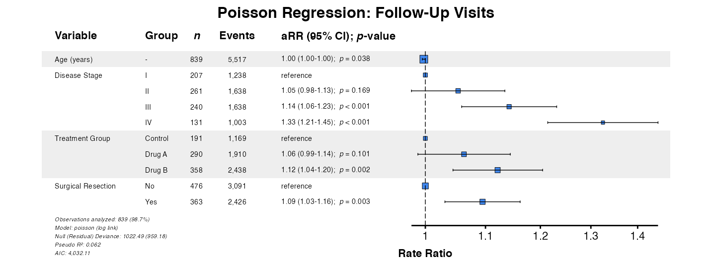

Example 22: Negative Binomial Regression

For overdispersed count outcomes (variance > mean), negative binomial regression is preferred. Using fit() ensures proper handling:

nb_result <- fit(
  data = clintrial,
  outcome = "ae_count",
  predictors = c("age", "treatment", "diabetes", "surgery"),
  model_type = "negbin",
  labels = clintrial_labels
)

example22 <- glmforest(
  x = nb_result,
  title = "Negative Binomial: Adverse Events"
)
queue_plot(example22)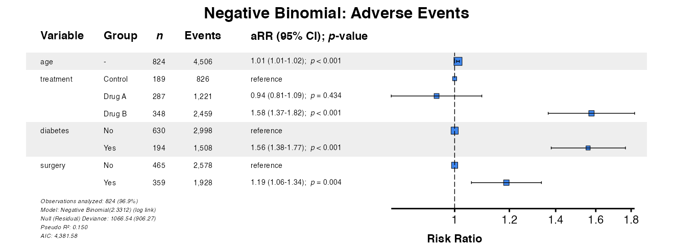

---

Function Parameter Summary

Parameter	Description	Default
x	Model object or model from fit() output	Required
data	Data frame (required for model objects)	NULL
title	Plot title	NULL
labels	Named vector for variable labels	NULL
indent_groups	Indent factor levels under variable names	FALSE
condense_table	Show binary variables on single row	FALSE
zebra_stripes	Alternating row shading	TRUE
show_n	Display sample size column	TRUE
show_events	Display events column (Cox models)	TRUE
digits	Decimal places for estimates	2
ref_label	Label for reference categories	"reference"
effect_label	Column header for effect measure	Model-dependent
color	Color for points and lines	Effect-type dependent
font_size	Text size multiplier	1.0
table_width	Proportion of width for table	0.55

---

Best Practices

Model Preparation

1. Ensure all factor levels are properly defined before fitting
2. Use meaningful reference categories
3. Consider centering continuous variables for interpretability
4. Check model convergence before plotting

Visual Design

1. Use indent_groups = TRUE for cleaner presentation of categorical variables
2. Match table_width to variable name lengths
3. Consider condense_table = TRUE for binary predictors
4. Use consistent colors across related figures

Publication Preparation

1. Use rec_dims attribute for optimal sizing
2. Save as PDF for vector graphics in print
3. Use 300+ DPI for raster formats
4. Check that reference lines and confidence intervals are clearly visible

---

Common Issues

Long Variable Names

If variable names are truncated, increase table_width:

p <- glmforest(model, table_width = 0.75)

Overlapping Text

Reduce font size or increase figure dimensions:

p <- glmforest(model, font_size = 0.9)
ggsave(file.path(tempdir(), "plot.pdf"), p, width = 14, height = 8)

Missing Labels

Ensure labels vector includes all variable names:

labels <- c(
  age = "Age (years)",
  sex = "Sex",
  stage = "Disease Stage"
)
p <- glmforest(model, labels = labels)

---

Further Reading

• Descriptive Tables: desctable() for baseline characteristics
• Survival Tables: survtable() for time-to-event summaries
• Regression Modeling: fit(), uniscreen(), and fullfit()
• Model Comparison: compfit() for comparing models
• Table Export: Export to PDF, Word, and other formats
• Multivariate Regression: multifit() for multi-outcome analysis
• Advanced Workflows: Interactions and mixed-effects models